Figure 1: In maximal Poisson-disk sampling disks cover the domain and ... The top-level grid provides an efficient way to test if a candidate dart is disk-free.
EUROGRAPHICS 2012 / P. Cignoni, T. Ertl (Guest Editors)
Volume 31 (2012), Number 2
A Simple Algorithm for Maximal Poisson-Disk Sampling in High Dimensions Mohamed S. Ebeida,1 Scott A. Mitchell,1 Anjul Patney,2 Andrew A. Davidson,2 and John D. Owens2 1 Sandia
National Laboratories of California, Davis
2 University
Figure 1: In maximal Poisson-disk sampling disks cover the domain and half-radius disks do not overlap. In 2d we generate 1 million points in 12 seconds (serial) and 1 second (GPU). The software is practical in up to 5d (serial) and 3d (GPU). Abstract We provide a simple algorithm and data structures for d-dimensional unbiased maximal Poisson-disk sampling. We use an order of magnitude less memory and time than the alternatives. Our results become more favorable as the dimension increases. This allows us to produce bigger samplings. Domains may be non-convex with holes. The generated point cloud is maximal up to round-off error. The serial algorithm is provably bias-free. For an output sampling of size n in fixed dimension d, we use a linear memory budget and empirical Θ(n) runtime. No known methods scale well with dimension, due to the “curse of dimensionality.” The serial algorithm is practical in dimensions up to 5, and has been demonstrated in 6d. We have efficient GPU implementations in 2d and 3d. The algorithm proceeds through a finite sequence of uniform grids. The grids guide the dart throwing and track the remaining disk-free area. The top-level grid provides an efficient way to test if a candidate dart is disk-free. Our uniform grids are like quadtrees, except we delay splits and refine all leaves at once. Since the quadtree is flat it can be represented using very little memory: we just need the indices of the active leaves and a global level. Also it is very simple to sample from leaves with uniform probability. Categories and Subject Descriptors (according to ACM CCS): Graphics—Computational Geometry and Object Modeling
1. Introduction Poisson-disk sampling is a sequential random process for selecting points from a subdomain. Each point must be diskfree, i.e. at least a minimum distance, r, from any previous point. For simplicity we consider constant r. The selected c 2011 The Author(s)
c 2011 The Eurographics Association and Blackwell PublishComputer Graphics Forum ing Ltd. Published by Blackwell Publishing, 9600 Garsington Road, Oxford OX4 2DQ, UK and 350 Main Street, Malden, MA 02148, USA.
Computing Methodologies [I.3.5]: Computer
points are called a sampling or distribution. The sampling is maximal if no more points can be added to it. The process for selecting points should ideally be bias-free: every uncovered point has a uniform chance of being selected next. This is equivalent to the probability of generating the next
Ebeida, Mitchell, Patney, Davidson, & Owens / A Simple Algorithm for Maximal Poisson-Disk Sampling in High Dimensions
point inside any disk-free subdomain being proportional to the subdomain’s area. This sampling process is crucial for many fields. In computer graphics, maximal Poisson-disk sampling (MPS) is desirable because the power spectrum of the inter-sample distances lacks low frequency noise, similar to blue noise. This pattern yields good visual resolution for rendering, imaging, texture generation, and geometry processing [PH04]. In ray tracing, Monte Carlo integration over importance samplings is used to capture soft shadows, motion blur, and depth of field. Combining a three dimensional scene with lighting and camera dimensions (e.g. shutter time) produces a high (e.g. five) dimensional space. MPS is also useful in the physical sciences for mesh generation, interpolation, and process modeling. In fracture mechanics, a mesh from a bias-free random point cloud keeps cracks from propagating along non-physical preferred directions [BS98, JB95]. MPS points produce simplicial and Voronoi meshes with provable quality [MTT∗ 96, EMD∗ 11, EM11]. Maximal distributions improve the efficiency and robustness of generating a mesh because the connectivity can be generated locally [AB04]. Stochastic collocation methods require high dimensional meshes with random positions and bounded quality [WI10, BNT10]. In chemistry and statistical physics, Poisson-disk sampling models random sequential adsorption [DWJ91]. The Poisson-disk process arises in nature and statistics, and is simple to describe. However, these do not immediately translate into a good algorithm, as we desire it to be fast, memory efficient, and parallel, and produce multidimensional points that are unbiased as well as maximal. 2. Algorithm Overview Our algorithm constructs a maximal d-dimensional Poissondisk sampling. Here we explain our technique at a high level, leaving the details for Section 4. The key to our technique is a simple data structure. Previous work used a dynamicallyconstructed quadtree/octree to keep track of uncovered regions of the domain. Such a data structure has comparatively large storage requirements and expensive operations for traversal, construction, and update. Instead we use an implicit “flat quadtree” data structure, which we explain below, that uses less memory. Our data structure keeps track of two things. First, as in prior work, we construct a base grid of uniform square boxes covering the domain we wish to sample. The base grid stores the samples. The grid cells are small enough that no cell can contain more than one sample. (Recall two samples have a minimum distance r between them.) Second, our “flat quadtree” lists the active subcells of the grid. It is this list of active cells that we refine, similar to a quadtree, as we iterate our algorithm. Unlike a quadtree, however, all the active cells are the same level and size. It is “flat” so we do not
need to store the tree and its pointers explicitly; instead, the index of each cell and the current iteration number (level) completely describes the cell. We initialize this list with the cells in the base grid and begin with iteration 0. At each iteration of the algorithm, we throw many darts into the list of active cells. For each dart, we pick a cell, then a point in the cell, both uniformly at random. We use the samples stored in the base grid to determine if the new dart is too close to an existing sample, in which case it is a “miss” and rejected. If the new dart passes the neighbor test, it is a “hit” and we add it to the sampling by (a) storing it in the base grid and (b) removing its bottom level cell from the list of active cells. At the end of the iteration, we refine each remaining active cell into 2d cells, e.g., in 2d squares become 4 smaller squares, as in a quadtree. Each new cell is tested against the sampling, and discarded if it is already covered by the disk of a single sample. Then we begin another iteration of the algorithm. We terminate the algorithm when no more active cells remain. Figure 2 shows sampling a unit square. GPU algorithm overview. Our algorithm is also amenable to parallel implementation; dart-throwing, neighbor tests, cell refinement and coverage tests, can all proceed in parallel. In parallel the only tricky part is ensuring accepted sample locations remain unbiased when parallel candidate darts conflict. Results overview. The process of generating points is provably bias-free, so the output is bias-free in practice. The distribution is maximal up to round-off error, meaning that every point of the domain is within distance r + ε of a sample point, where ε is the numerical precision. We observe linear run-time in output size n for a given d. This is because in practice the fraction of darts throws that are hits is a constant. The runtime is the finite sum of an infinite geometric series independent of the maximal grid level. Our number of quadtree levels is bounded by the bits of precision. Deep levels are needed to resolve certain “unlucky” cases of several disks that together cover a cell, but no one disk covers the cell by itself. For us these are rare enough they can be handled without a level limit or any special effort to detect them. Our serial implementation samples one million points in about 10, 90, and 1400 seconds in 2d, 3d and 4d respectively. Using 2 GB of memory on a modern laptop, we generated samplings of 24, 6, and 1.4 million points in 2d, 3d and 4d. Although efficiency degrades with dimension, we were able to sample 300k points in three hours in 5d, and 44k points in 80 minutes in 6d. We believe these are the largest d-dimensional bias-free maximal Poisson-disk distributions in the current literature. We also demonstrate parallel GPU implementations in 2d and 3d. On an NVIDIA GTX 460, we can generate 600,000 samples at a rate of 1,000,000 samples/second in 2d, and c 2011 The Author(s)
c 2011 The Eurographics Association and Blackwell Publishing Ltd.
Ebeida, Mitchell, Patney, Davidson, & Owens / A Simple Algorithm for Maximal Poisson-Disk Sampling in High Dimensions
200,000 samples at 75,000 samples/second in 3d. The size limitations are due to 1 GB of memory. 3. Previous Work
(a) Iteration 0 End
(b) Iteration 1 Start
(c) Iteration 1 End
(d) Iteration 2 Start
(e) Iteration 2 End
(g) Iteration 3 End
(f) Iteration 3 Start
(h) Iteration 4 Start
Figure 2: Example sampling of a unit square with r = 0.2. Active cells are light, inactive are dark. The right-hand column shows the active cells at the start of an iteration. The left-hand column shows the cells remaining in the active cell list before they are subdivided. Some active cells are already covered by a single disk, but it is more efficient to leave them until they are selected or the end of the iteration. In this example we detected that the sampling is maximal at the beginning of iteration 4, because there are no active cells. c 2011 The Author(s)
c 2011 The Eurographics Association and Blackwell Publishing Ltd.
During the last decades many methods were proposed to generate maximal Poisson-disk samplings. The classical dart throwing algorithm [DW85,Coo86] produces unbiased diskfree points, but requires unbounded time to achieve a maximal distribution. A bias-free dart is thrown and rejected (a “miss”) if it is closer than the minimum distance required to a previous successful dart, otherwise it is accepted (a “hit”). As more darts successfully hit the domain, the remaining uncovered parts of the domain (“voids”) get smaller, decreasing the probability of acceptance. In order to improve the efficiency, many methods were proposed to solve a relaxed version of the problem. Some methods sacrificed the biasfree condition: Wang tiles [CSHD03, LD05] and Penrose tiles [ODJ04, Ost07], for instance, do not target the whole domain uniformly when a dart is thrown; other methods have the same behavior [Mit87,Jon06,DH06,Bri07] for other reasons. For example, Jones picks a sampling sub-region based on the relative area of some Voronoi cells covering the domain. This introduces bias: a relatively large Voronoi cell, with higher selection probability, might contain a relatively small void. Wei’s parallel sampling method [Wei08] used a sequence of multi-resolution uniform grids, but its output distribution is biased and only near-maximal. Bowers et al. [BWWM10] use a similar phase-group-decomposition method to Wei, but without a hierarchy. Output quality is typically evaluated using the Fourier transform, radial anisotropy, and radial mean power plots. Tiling methods are fast, but the bias in their output can be observed in these pictures. Some advancing front methods are fast, and in some cases their bias is not visible using these pictures. Unfortunately, the community currently lacks a definitive test of whether a (biased) process produces acceptable output; PSA [Sch11] is a start for 2d. For this reason we concentrate our attention on methods whose process is unbiased. Some methods follow a bias-free sampling process and achieve maximality within some threshold. The ones most directly related to this paper are by White et al. [WCE07], which is 2d only; and Gamito & Maddock [GM09], which extends to higher dimensions. They throw darts in sequence, discarding or keeping one depending on whether it is covered by a prior dart’s disk. The improvements over classic dart throwing come from retrieving prior darts locally using a uniform grid, and refining that grid in a quadtree to track and target the remaining disk-free area. The diagonal of a top-level grid square is equal to the sampling radius, so each square accepts at most one dart. To throw an unbiased dart, a quadtree leaf is selected weighted by its area, then a dart is selected uniformly from within it. The likelihood that the dart is a hit (disk-free) is equal to the ratio of the disk-free
Ebeida, Mitchell, Patney, Davidson, & Owens / A Simple Algorithm for Maximal Poisson-Disk Sampling in High Dimensions
area within a square, to the area of the square itself. There is no a priori bound on the ratio, but if a miss occurs, the square is refined to better capture the disk-free area. Subsquares covered by prior disks, or smaller than some threshold, are discarded. The threshold affects maximality and bias. The authors claim that empirically the number of boxes, m, is O(n), which may include some threshold- and dimensiondependent constants. Recently we reported a provably correct variation [EPM∗ 11]. It uses the same top-level grid but, instead of a quadtree, a direct representation of the disk-free regions. We compute the points of intersection between a square and nearby circles, and those circles with one another. The points define a convex polygonal void which is a provably-tight outer-approximation to the local disk-free region. The likelihood of a miss is bounded by a constant, and there are O(n) voids. This yields an algorithm using O(n) space and E(n log n) time, and the output is provably maximal and bias-free. The method is described in two dimensions; in theory it may extend to higher dimensions but constructing non-convex polyhedral voids would be complicated in practice. Most methods are inherently discrete and sequential, in that darts are produced and resolved one at a time. Jones and Karger [JK11] depart from this paradigm by directly modeling the time of arrival of points following the Poisson process. The same top-level grid is used, but each square computes the location and time of arrival of its first point independently. Then the arrival times of conflicting points in nearby squares are resolved sequentially. If points conflict, the later point is rejected and the time and location of the next-arriving point is generated if needed. It would be interesting to do an empirical evaluation of the work and memory spent generating and updating the times of unused points, and compare it to the work sequential methods spend on quadtrees, voids, and dart misses. Other Poisson-disk sampling implementations on the GPU include Ebeida et al. [EPM∗ 11], Bowers et al. [BWWM10] and Wei [Wei08]. The traditional domain is the unit square, cube, . . . , ddimensional box. Periodic boundary conditions, i.e. the domain is a d-dimensional torus, are used to remove boundary effects when empirically measuring bias. Some prior work addresses more complicated domains, such as 2-dimensional polygons with holes [EPM∗ 11]. 3.1. Comparison to Related Work Compared to our method, Wei [Wei08] is faster, but the sampling is not maximal. White et al. [WCE07] is unbiased, maximal and faster, but is 2d only and uses more memory. We use an order of magnitude less memory than the prior unbiased methods [GM09, EPM∗ 11], but use some
of the ideas of each. We use the top-level uniform grid G o for checking disk-overlap in constant time as in Ebeida et al. [EPM∗ 11]. Samples are guided by grids similar to Gamito & Maddock’s [GM09] quadtree, but uniformly refined to the same level at any given time. Our algorithm proceeds through a series of iterations throwing a fixed number of darts, as the Phase stages II of Ebeida et al. [EPM∗ 11]. Our flat quadtree has several advantages. Except for the top level base grid, the cells are all implicit. There is no datastructure for a cell: no tree or pointers [GM09], no polygons [EPM∗ 11]. We need only store spatial indices, d integers, for each cell. Even these indices only exist for the subset of cells not yet covered by disks. Gamito & Maddock use one array per quadtree level, whereas since we only have one level at a time we can pack data more efficiently into a single array. This results in lower storage requirements by an order of magnitude. In practice our memory in d + 1 dimensions is about the same as Gamito & Maddock’s or Ebeida et al.’s in d, so one could say we get one dimension “for free.” Since the cells all have the same area, it is simple to select one in constant time without bias. In contrast, both quadtrees and polygonal voids have varying area, so some sort of binary search is needed. Ebeida et al. in Phase II takes log |G o | = log n time to select a polygon. In Gamito & Maddock, all the cells of a given level have the same area, so one could select a level in O(log(max level)) time then select a quad of the level in O(1) time. In all these methods, in practice the non-constant selection time is dominated by the O(1) expense of checking each dart for a miss and refining the quadtree or constructing each void. In Gamito & Maddock, the hit rate improves locally as a cell with a miss is refined to better approximate the uncovered area. For us, we refine cells in lock-step after the fixed number of throws in an iteration. In Figure 5 we see a constant hit rate after the first few iterations; explicitly tracking where the misses occur is not necessary. In 2d we have about the same running time as Ebeida et al. and we are an order of magnitude faster than Gamito & Maddock in dimensions up to 5. Using simpler datastructures that change less often not only saves memory, it is also faster. 4. Algorithm Details Algorithm 1 presents pseudocode for the serial algorithm. Now we describe the important implementation nuances. Base grid. The uniform base grid, G o , covers the domain. Cells are sized so that a cell can accommodate at most one point: √ diagonals are r, which means the side lengths are so = r/ d. (Side lengths shrink with the dimension.) Each base grid cell stores a single sample or is empty. We consider cells to be open on their minimal extremes, half-open squares. This ensures that a point is assigned to a unique base cell, and dart generation is not biased towards the boundary between active cells. c 2011 The Author(s)
c 2011 The Eurographics Association and Blackwell Publishing Ltd.
Ebeida, Mitchell, Patney, Davidson, & Owens / A Simple Algorithm for Maximal Poisson-Disk Sampling in High Dimensions
Work
Bias-free
Maximal
Compute bound
Memory bound
Classic dart-throwing [DW85, Coo86] Voronoi [Jon06] Scalloped sectors [DH06] Hierarchical dart throwing [WCE07] ? Parallel multi-resolution uniform grid [Wei08] Spatial subdivision [GM09] ? 2-phase [EPM∗ 11] ‡ Point arrival times [JK11] ‡ This work?
yes no no yes no yes yes yes yes
no yes no yes no yes yes yes yes
∞ n log n n log n n n n† n log n n n
n n log n n n n n† n n n
?
These methods all use quadtrees to guide dart-throwing and represent uncovered areas. The paper claims O(n log n) runtime and O(n log n) memory, but we interpret their tree size to be O(n), with some d and level threshold dependence. ‡ Provable bias-free process, maximal output, and compute and memory bounds. Others’ bounds are empirical.
†
Table 1: A comparison of Poisson-disk methods. Many have similar asymptotic complexity in n, but few explain their dependence on dimension d or bits of precision b. Memory dependence on d and b is critical in practice.
Algorithm 1 Simple MPS algorithm, CPU. initialize G o , i = 0, C i = G o while |C i | > 0 do {throw darts} for all A|C i | (constant) dart throws do select an active cell Cci from C i uniformly at random if Cci ’s parent base grid cell Gco has a sample then remove Cci from C i else throw candidate dart c into Cci , uniform random if c is disk-free then {promote dart to sample} add c to Gco as an accepted sample p remove Cci from C i {additional cells might be covered, but these are ignored for now} end if end if end for {iterate} for all active cells C i do if i < b subdivide Cci into 2d subcells retain uncovered (sub)cells as C i+1 end for increment i end while
Active cells. Each cell is uniquely defined by d integer indices and the level l. Cells at level l have spacing 2−l × so . Any cell can identify its parent in constant time via simple integer operations. Besides the indices, there is no datastructure for a nonbase cell. Inactive cells require no storage. We store the indices of the active cells in separate arc 2011 The Author(s)
c 2011 The Eurographics Association and Blackwell Publishing Ltd.
rays, one for each of the d dimensions. However, a twodimensional array of width d could be used instead. These arrays are fixed length, and are used for all iterations. Update in place. We wish to make the arrays long enough to accommodate cell division at the end of an iteration, without dynamic memory allocation. We use arrays of length B|C o |, where B is a dimensional-dependent constant. In practice, we have found that a value of B = d works well. During an iteration the cell lists only decrease, so it is sufficient to ensure that the number of active cells is less than B|C o | at the start of an iteration. In an iteration we throw A|C i | darts, where A is another dimensional-dependent constant. We have chosen A large enough that many fewer than 2d subcells are uncovered on average. See Section 4.2 below. Coverage and disk-free checks. We identify nearby cells using a template of base-grid index offsets. It is precomputed before √ any of the iterations. The template is a subset of a d2 d + 1ed lattice of cells: those cells with a corner closer than r to a corner of the center cell. Winnowing the lattice reduces the template significantly as the dimension increases. When checking if a dart is disk-free, or a cell is covered, only the samples in the template cells around the parent base-grid cell are relevant. For efficiency, cells closest to the center cell are checked first, as their samples are more likely to cover the dart or cell. To check if a dart is disk-free, we check if it is farther than r from every nearby cell sample. To check if a cell is covered, we check if all of its corners are covered by any one nearby cell sample. All the 2d subcells can be checked at once by checking 3d points. See Figure 3. Since a cell might be completely covered by a combination of disks of several nearby darts, but not by a single disk,
Ebeida, Mitchell, Patney, Davidson, & Owens / A Simple Algorithm for Maximal Poisson-Disk Sampling in High Dimensions
ent construction of the base grid may be necessary to ensure the memory and runtime are linear in the output size.
!"
&" %"
!#$"
(a) Covered cell
!$# %$# !"# %"#
%&# %'#
!$#
(b) Uncovered cell with covered children
Figure 3: (a) Cell C is covered because its farthest corner is less than is ≤ r + ε away from disk-center p . (b) When a cell is split, we check whether each of its children are covered.
being “uncovered” does not guarantee that there exists some available region for sampling. We experimented with using the square-inside-circle test of White et al. [WCE07]. This can detect whether a cell is covered by multiple disks by checking if all of its potential children (grandchildren, etc.) are covered by single disks. However, these tests added code complexity without improving the average performance. Level limit. Iteration i uses grid level l = min(i, b) where b is the bits of precision in our floating point numbers. The algorithm becomes slightly simpler when the quadtree level reaches the maximum. Each half-open C b cell holds a single d-dimensional floating-point number. The multiple-disk coverage problem is resolved. Advancing to the next iteration involves merely discarding the current cells (which are just points) that are inside a (new) disk. We use integer indices to represent cells, which are converted into floating point boxes when placing darts. A level limit of 23 corresponds to boxes about 1e-7 the width of the base grid boxes. The sampling is maximal up to the diagonal of the smallest boxes, de-7×so . 4.1. General Domains The algorithm description and analysis assumes that the domain is a unit box, and that each cell is entirely interior to the domain. This requirement may be relaxed by a simple amendment: treat the exterior of the domain as previous disk-covered areas. We require a primitive that returns whether a candidate dart is exterior to the domain, and an oracle to tell whether a domain boundary cuts a box. For many solid modeling engines the runtimes of the primitive and oracle are significant. Also more miss-darts will be thrown, especially if the domain has thin regions. In some cases the effect of the misses can be bounded by the finite precision because small enough boxes will be entirely interior or exterior to the domain. For a domain whose volume is significantly smaller than the volume of its bounding box, a differ-
4.2. Complexity Our algorithm has two tuning constants, A and B. A determines the number of throws, and B determines the length of the arrays storing the active cells. They are interdependent and their relative values determine a memory—speed tradeoff. These tuning parameters were determined empirically. 1. Speed: smaller A (larger B) is faster. 2. Storage: larger A (smaller B) uses less memory. If we throw more darts during an iteration, a larger fraction of them will be misses, slowing down the algorithm. The miss-fraction increases because of several reasons. As an iteration progresses the voids get smaller but the cells approximating them are fixed size. A cell might have no void at all because it is completely covered by a combination of several disks, but still be active because it is not covered by a single disk. When a dart hits, it might completely cover some other cells, but we do not remove them immediately because searching would take too much time. (To simplify the overview, all active cells with the same parent were discarded in Figure 2.) If we throw more darts, we will get more hits, and there will be fewer active cells (and fewer uncovered subcells) at the end of an iteration. Indeed, we need A larger than a threshold so that the number of subcells decreases from one iteration to the next. In the first few iterations, the number of active subcells actually grows. But once the active cells are small and the uncovered regions are isolated, the number of subcells decreases geometrically. See Figure 5. According to our numerical studies, picking A ∈ [0.3, 0.6] for dimensions 2 and 3 balances these two factors well. A = 0.8 works well for d = 4. In our experience the performance is not sensitive to the exact value of A above the threshold. For higher dimensions it appears that the threshold increases dramatically, e.g. A = 10 for d = 5. For a given dimension, we have chosen to fix B and find a sufficiently large value of A. It is possible that increasing B may help reduce A, but will have little effect on the threshold. A variation would be to use an adaptive value of A. When refining cells, if the number of uncovered children exceeds the current memory, de-refine (or recompute) the cells and continue to throw more darts in the current iteration. 4.2.1. Linear Time Most of the time is consumed during the first few iterations. These generate most of the darts. After that, the number of active cells decreases from iteration to iteration by a constant factor, c2 . Empirically c2 ≈ 0.5 for our choice of A, see Figure 5. This provides the intuition for why we achieve c 2011 The Author(s)
c 2011 The Eurographics Association and Blackwell Publishing Ltd.
Ebeida, Mitchell, Patney, Davidson, & Owens / A Simple Algorithm for Maximal Poisson-Disk Sampling in High Dimensions
expected linear running time. Each dart throw takes constant time, so iteration i takes c1 |C i | work. If we include the dimensional-dependent factors, the template size and the √ number of coordinates, then c1 = Add2 d + 1ed . i |C o | = Θ(n) [EPM∗ 11]. The total work w = c1 ∑∞ i=0 |C |, i+1 i and |C | < c2 |C |, so the infinite geometric series sum is w = |C o |c1 /(1 − c2 ) = E(nd 1+d/2 ). The algorithm will terminate at iteration log1/c2 |C o | and the total work is linear in |C o |, just as a binary tree has log2 n depth and 2n size.
Since log1/c2 (|C o |) is a very slowly growing function of |C |, only a handful of darts are added after iteration 16 for even our largest samplings. In order to resolve cells that are covered by multiple disks that just barely overlap, we often iterate to i = b = 23. These are such a small fraction of the total number of cells that they do not effect our running time or memory needs. (This is in contrast to Gamito & Maddock [GM09], where cells with misses are refined immediately, and the paper claims that an explicit level limit, e.g. 16 � 23 = b, is required to avoid a blow-up in the number of active cells.) o
We have been unable to derive provably optimal, or even necessary and sufficient values, for A and B. Nor are we able to prove the expectation that |C i+1 | < c2 |C i |. To do so would require spatial statistics theorems bounding the average fractional area of a active cell covered by prior disks, and the average-case number of child cells that are not completely covered by a disk. 4.2.2. Linear Memory Given dimension d and bits of precision b, our memory is O(bdBn) = O(d 2 bn). The output sample points require nbd bits: n points with d coordinates with b bits. The grid cells require O(Bndb) bits: each cell has d indices with b bits; the number of cells is O(Bn), which hides some dimensional dependence on the sampling density and ignores any domain boundary effects.
The dart-throwing part of our GPU implementation closely follows the work by Ebeida et al [EPM∗ 11]. Algorithm 2 Simple GPU MPS algorithm. PARALLEL are GPU kernels, SERIAL are CPU steps. initialize G o , i = 0, C o = G o , as Algorithm 1 while |C i | > 0 do {SERIAL} {throw candidate darts, in parallel} for all A|C i | threads do {PARALLEL} select an active cell Cci from C i uniformly at random reject if parent base grid cell Gco is locked throw candidate dart c into Cci uniformly at random if c is disk-free w.r.t. accepted darts {p} then lock Gco save c and its arrival index as a candidate in Gco end if end for {accept first candidate darts, in parallel} for all base grid cells G o without an accepted sample do {PARALLEL} if cell Gco has a candidate c then if c is disk-free w.r.t. candidate darts {c} with a lower arrival index then promote dart c to sample p, updating Gco and C i as Algorithm 1 else mark Gco for unlocking before next iteration end if end if end for {generate subcells in parallel} for all active cells C i do {PARALLEL} if i < b subdivide Cci into 2d subcells append uncovered (sub)cells to the list C i+1 end for increment i {SERIAL} end while
4.3. GPU Implementation Details
5. Experimental Setup and Results
Our algorithm can be extended to parallel platforms. To demonstrate this, we implemented GPU versions in 2d and 3d. We used NVIDIA CUDA 3.2 on an NVIDIA GTX 460 GPU. Algorithm 2 provides an overview.
Memory and time. Figure 4 compares the running time and memory usage of our algorithm to Gamito and Maddock’s [GM09] in 2, 3 and 4 dimensions, and to Ebeida et al.’s [EPM∗ 11] in 2 dimensions. See also Eurographics2012 Additional Material Appendix A Figure 8 for a linear scale.
There are three main parallel steps: generating candidate darts, checking that they are disk-free, and subdividing and keeping uncovered cells. To avoid race conditions, disk-free checks are performed in two parallel stages: once against previously accepted samples, and once against current candidate darts. If candidate darts conflict, the ones with higher arrival indices are rejected. Parallel selection causes a larger fraction of the thrown cells to be misses than in the serial case, the price we pay for parallelism. We use the index of the thread generating the dart as its arrival index. This does not add bias, since threads randomly pick cells. c 2011 The Author(s)
c 2011 The Eurographics Association and Blackwell Publishing Ltd.
It appears that we use a factor of 8 less time and a factor of 2–3 less memory than Gamito and Maddock in 2 dimensions. In 3 dimensions the factors are 9–10 for time and 4–5 for memory. In 4d, the factors are 6–8 (for A = 0.6–1.6) for time and 10 for memory. We are able to go one dimension higher given the same time and space bounds. In 2 dimensions, we use about the same runtime as Ebeida et al., but a factor of 2–3 less memory. Gamito and Maddock’s Figure 4 [GM09] shows both the
Ebeida, Mitchell, Patney, Davidson, & Owens / A Simple Algorithm for Maximal Poisson-Disk Sampling in High Dimensions
d
A
B
n
r (×10−4 )
so (×10−4 )
|G o |
MC (GB)
M (GB)
t = runtime (s)
n/t
m/n
2 3 4 5 6
0.3 0.3 0.6 10 700
2 3 4 5 6
24M 6.1M 1.4M 340k 44k
1.7 50 280 830 3100
1.2 28 140 370 1300
69M 43M 25M 14M 0.26M
1.1 1.0 0.80 0.56 0.012
2.1 1.9 1.8 1.6 0.017
330 700 1900 10000 4800
73000 8600 760 33 0.93
4.7 19 140 5800 560000
Table 2: CPU performance statistics for our largest samplings by dimension d. A is the number of throws per initial active cell; B is the dimensional-dependent constant that governs the amount of memory used; n is the output size; r is the Poisson-disk radius; so is the base grid side lengths; G o is the base grid; MC is the amount of memory that stores active cell indices while M is the total amount of memory; and m is the total number of dart throws, including misses. The last two columns give the relative efficiency by dimension: samples per second, and throws per successful dart.
%476$
!"#$%&'*&'546$%1/7#'829':1#"231$2'
!"#$%&'()*+'
)*+,-.$(&$
!"#$%&$ !"#$(&$ !"#$'&$ )*+,-.$'&$ )*+,-.$%&$ /01,2*$%&$
346($ !"#$%&$ !"#$'&$ !"#$(&$ 3456$
)*+,-.$%&$ )*+,-.$'&$ )*+,-.$(&$
343($ 3435$
/01,2*$%&$ 343($ 3456$ 346($ %476$ ,-#*"%'$.'$-/0-/'0$12/3'(#1441$23+'
534%($
(3486$
!"#$%/5%647)0"28#%9*+%:"#$*'")*%
!"#$%&'$()*+',%
36%($
)*+,-.$(&$
!"#$(&$ )*+,-.$'&$
)*+,-.$%&$ !"#$'&$
%54$
!"#$%&$
4($
34$ /01,2*$%&$ ($ 6763$
676($
!"#$%&$ !"#$'&$ !"#$(&$ )*+,-.$%&$ )*+,-.$'&$ )*+,-.$(&$ /01,2*$%&$
6734$ 674($ %754$ 367%($ -.#/$0%)1%).23.2%3)"*2'%&#"44")*',%
(6784$
Figure 4: Memory and time of our algorithm vs. bias-free alternatives. Log–log scales with 0-intercept trendlines.
runtime and memory challenges in efficiently generating a fixed-size sampling as the dimension increases; our results in Figure 4 across dimension are consistent with these trends. While the complexity is roughly linear in output size for all of the methods we considered, including ours, the dependence on dimension was severe and appears fundamental.
For any fixed dimension, as long as A is above a threshold, its effect on the runtime is rather mild; see Eurographics2012 Additional Material Appendix A Figure 9. However, as the dimension increases, the miss rate increases and the number of uncovered subcells per cell increases. To stay within the memory budget, A must be increased. Table 2 gives performance details by dimension. For example, the last column illustrates the increasing miss rate. Figure 5 shows that the challenges grow with dimension in the first few iterations, but for later iterations the algorithm performs about the same regardless of dimension. In 5 dimensions we generated 340,839 points in 2.8 hours and 1.5 GB of memory. We threw 1.9 billion (1.9e9) darts. Using B = d = 5, we had to increase A from 0.6 to 10 for the subcells to fit in their array. GPU results. Our GPU implementations, run on a midrange NVIDIA GTX 460, are able to achieve 1M samples per second in 2d, and 75k samples per second in 3d. This is about a 10× speedup over our CPU implementation. The available memory allows us to produce about 600k points in 2d, and 200k points in 3d. Bias-free. Our serial process is provably bias free. By selecting an active cell uniformly then selecting a point in the cell uniformly, the probably of introducing the next part within any disk-free region is proportional to the area of that region. This is equivalent to bias-free [EPM∗ 11]. To demonstrate that the output is bias-free, we present radial mean power and anisotropy variations for an averaged collection of ten sampling patterns. These plots, shown in Figure 6, follow expected blue noise behavior and match past literature [WCE07, Wei08]. The anisotropy measure indicates a consistent drop of 10 dB across the spectrum for ten distributions. For our GPU implementation, we show slices of the 3d FFTs based around the XY, YZ and XZ axes in Figure 7. We see the expected noise, with no artifacts in any dimension. See also Eurographics2012 Additional Material Appendix A Figure 10. These confirm that output is biasfree. c 2011 The Author(s)
c 2011 The Eurographics Association and Blackwell Publishing Ltd.
Ebeida, Mitchell, Patney, Davidson, & Owens / A Simple Algorithm for Maximal Poisson-Disk Sampling in High Dimensions ,)*$"$-"./01'("$-"23*4'"&$"5)6'"7(89":';;6"" 46