154
IEEE SIGNAL PROCESSING LETTERS, VOL. 15, 2008
A Simple and Accurate Algorithm for Barycentric Rational Interpolation Luc Knockaert, Senior Member, IEEE
Abstract—A very simple non-iterative signal approximation scheme based on rational barycentric interpolation and the null-space of a Löwner matrix is presented. Numerical examples demonstrate the accuracy and robustness of the approach.
and denominator (without common with numerator zeros) of exact degree less than . Then, given distinct interpolation nodes , we can form the Lagrange interpolants [17]
Index Terms—Barycentric interpolation, Lagrange interpolation, null-space, rational functions, signal representation.
(2)
I. INTRODUCTION
(3)
HE PROBLEM of rational approximation and interpolation arises quite naturally in signal processing [1], numerical analysis [2], and system identification [3]. The amount of literature concerning the topic of rational approximation and interpolation is therefore quite huge. With regard to rational approximation techniques, we have Padé approximation [4], uniform Remes approximation [5], curve fitting [6], [7], and the related vector fitting [8] approaches. With regard to rational interpolation, we have the Bulirsch–Stoer method [9], the Neville-type interpolation [10], and Thiele continued fraction interpolation [11]. A large number of the above approaches, but this is not exhaustive, are documented in Grosse’s catalog [12]. A generally lesser known, though still well-documented, interpolation technique is barycentric interpolation [13]–[16], which bears a close relationship with Lagrange interpolation [17] and its potential multivariate extensions [18]. In this letter, we present a very simple interpolation scheme based on rational barycentric interpolation and the null-space of a Löwner [19], [20] matrix. Pertinent numerical simulations demonstrate the accuracy and robustness of barycentric Löwner-based interpolation, which moreover presents the advantage of being a non-iterative approach.
T
II. BARYCENTRIC RATIONAL INTERPOLATION
where (4) This results in the following expression for
: (5)
Defining the weights
as (6)
it is seen that
can be written in the barycentric format (7)
Now, any other choice of the weights, say, rational function
, results in a
(8) such that
The idea is the following: suppose we are given a rational function (1) Manuscript received July 31, 2007; revised October 1, 2007. The associate editor coordinating the review of this manuscript and approving it for publication was Prof. Yue (Joseph) Wang. The author is with the INTEC-Ghent University, B-9000 Gent, Belgium (e-mail:
[email protected]). Color versions of one or more of the figures in this paper are available online at http://ieeexplore.ieee.org. Digital Object Identifier 10.1109/LSP.2007.913583
interpolates at the node set , i.e., . Even more important, for any given smooth function (see also Theorem 1 of the Appendix), one excan readily find a rational function which interpolates , namely, the barycentric rational actly at the nodes interpolant [13]–[16] (9) where the weights can be freely chosen. A pertinent error analysis regarding the barycentric scheme (9) is given in the Appendix. Three specific ways for choosing the weights can be distinguished.
1070-9908/$25.00 © 2008 IEEE
KNOCKAERT: SIMPLE AND ACCURATE ALGORITHM
155
A. Degree Selection Fix the exact degree of the numerator and denominator of and a expression (9), i.e., select a numerator degree denominator degree , with , such that (10) The un-normalized unknowns are clearly and . This approach has been described in [13] and [14]. Note that the case is just plain polynomial Lagrange interpolation [17]. B. Pole Selection It is easily seen that the poles of the equation
are found by solving
(11) for . We will give an efficient way of solving equation (11) in the sequel. If one fixes the poles , we can find the vector of weights in the null-space of the Cauchy matrix [19] (12)
Lebesgue constants [21], it is known that the extended Chebyshev nodes are a near-optimal choice. If we fix the approxima, the extended Chebyshev nodes are tion range as (16) . for Remark: In signal processing, most measured observations are physically obtained at equidistant nodes. In order to retain the advantage of the extended Chebyshev nodes, we recommend replacing the measured data with a smooth interpolant, such as cubic spline, calculated at the Chebyshev nodes. The null-space of the Löwner matrix (14) is calculated by , which means of the SVD-based MATLAB® function generates an orthonormal basis for the null-space.1 In order to find the poles of the rational barycentric approximation, we must solve (11) efficiently. We base our approach on a result of the diagonal in [22] which states that the eigenvalues matrix are the roots of minus rank-one the secular equation (17) Multiplying (11) by , we obtain that the poles lutions of the equation
must be so-
This and similar approaches are treated in [15] and [16]. (18) C. Test Node Selection Since interpolants in general tend to fluctuate enormously between the interpolation nodes, we may choose the weight vector such that the interpolation error vanishes at some judiciously test nodes . Of course, we chosen set of must require that for . Therefore, we impose the additional constraints
where the trivial simple pole at 0 must be discarded. As we do not want to allow poles at infinity, we require . It is seen by inspection of the secular (17) that the solutions of , where (18) are the eigenvalues of the matrix (19) Note that the zeros are obtained by solving
(13) This means that the weight vector must belong to the nullLöwner matrix [19] space of the
(20) which is similar to (11). Letting (9), the gain is found as
tend to infinity in expression
(21)
(14) A similar procedure, but with the test nodes a selected subset of the original nodes, has been proposed in [20].
resulting in an easily found pole-zero-gain format for the barycentric rational approximation. A. First Example
III. NUMERICAL PROCEDURE AND EXAMPLES Here, we opt for test node selection and choose the test nodes at the midpoints. In other words, we put (15) We also have to select the nodes themselves. From node selection theory for Lagrange interpolation in connection with the
As a first example, we take the rational function
(22) 1The null-space may contain more than one vector, in which case we select the lexicographically most significant one.
156
IEEE SIGNAL PROCESSING LETTERS, VOL. 15, 2008
Fig. 1. Logarithmic error for the first example.
Fig. 2. Logarithmic error in the presence of a double pole.
with . Note that may represent the angular frequency , where is the Laplace transof the real-rational function form variable. The logarithmic error for barycentric rational interpolation with six extended Chebyshev nodes is shown in Fig. 1. Note that the method is quite stable in the presence of by introducing multiple poles. For example, if we modify a double pole, i.e.,
(23) we find that the logarithmic error for barycentric rational interpolation with seven extended Chebyshev nodes as shown in Fig. 2 is still very small. Fig. 3. Logarithmic error for the second example.
B. Second Example As a second example, we take the function (24) which represents a unit delay in the Laplace transform domain. The logarithmic error for barycentric rational interpolation with 13 extended Chebyshev nodes is shown in Fig. 3. Note that is a rational approximation for the unit delay with 12 zeros and 12 poles. Since in general the number of nodes can be freely chosen, it might be good in practice to determine adaptively such that the overall absolute error is below a previously selected threshold.
space of a Löwner matrix. Numerical simulations have demonstrated the accuracy and robustness of the method, while a pertinent error analysis and the transformation to the more usual pole-zero-gain format were also discussed.
APPENDIX ERROR ANALYSIS Given a sequence of distinct nodes and non-vanishing weights , we define two discrepancy measures, namely
IV. CONCLUSION We have presented a very simple non-iterative interpolation scheme based on rational barycentric interpolation and the null-
(25)
KNOCKAERT: SIMPLE AND ACCURATE ALGORITHM
157
(26)
and
Note that and following theorems. Theorem 1: Let
, while . We can now state the
(27) be the barycentric interpolant of the . Then interval
function
over the
(28) where
is the uniform norm over , i.e., (29)
Proof: We have (30) By the mean value theorem, this can be written as (31) where the points are inside , and hence, the proof follows. Theorem 2: Let be the vector and let the condition number [23] of the barycentric interpolation be defined as
(32) where the inequalities between vectors are interpreted componentwise. Then (33) where stands for componentwise multiplication. Proof: Similar to the proof in [23] for barycentric Lagrange interpolation. Note that the first Theorem controls the absolute error over the interval , while the second Theorem controls the relative error . due to inaccuracies (and/or noise) on the function values
In both cases, the errors are out of control whenever some of the poles of the barycentric interpolation are located inside the interval . This, however, never happened in our simulations. REFERENCES [1] P. Stoica and R. L. Moses, Introduction to Spectral Analysis. Englewood Cliffs, NJ: Prentice-Hall, 1997. [2] A. Cuyt and L. Wuytack, Nonlinear Methods in Numerical Analysis. Amsterdam, The Netherlands: North-Holland, 1987. [3] R. Pintelon, P. Guillaume, Y. Rolain, J. Schoukens, and H. Van Hamme, “Parametric identification of transfer functions in the frequency domain-a survey,” IEEE Trans. Autom. Control, vol. 39, no. 11, pp. 2245–2260, Nov. 1994. [4] J. C. Mason, “Some applications and drawbacks of Padé approximants,” in Approximation Theory and Applications.. New York: Academic, 1981. [5] Y. L. F. Chiang, “A modified Remes algorithm,” SIAM J. Sci. Stat. Comp., vol. 9, pp. 1058–1072, 1988. [6] E. C. Levi, “Complex curve fitting,” IRE Trans. Autom. Control, vol. AC-4, pp. 37–44, 1959. [7] C. K. Sanathanan and J. Koerner, “Transfer function synthesis as a ratio of two complex polynomials,” IEEE Trans. Autom. Control, vol. 8, no. 1, pp. 56–58, Jan. 1963. [8] W. Hendrickx and T. Dhaene, “A discussion of ‘Rational approximation of frequency domain responses by Vector Fitting,” IEEE Trans. Power Syst., vol. 21, no. 1, pp. 441–443, Feb. 2006. [9] J. Stoer and R. Bulirsch, Introduction to Numerical Analysis. New York: Springer-Verlag, 1980. [10] W. H. Press, W. T. Vetterling, S. A. Teukolsky, and B. P. Flannery, Numerical Recipes in C++: The Art of Scientific Computing, 2nd ed. Cambridge, U.K.: Cambridge Univ. Press, 2002. [11] M. Abramowitz and I. A. Stegun, Handbook of Mathematical Functions with Formulas, Graphs, and Mathematical Tables, 9th Printing.. New York: Dover, 1972, p. 881. [12] E. Grosse, , J. C. Mason and M. G. Cox, Eds., “A catalogue of algorithms for approximation,” in Algorithms for Approximation II.. London, U.K.: Chapman & Hall, 1990, pp. 479–514. [13] C. Schneider and W. Werner, “Some new aspects of rational interpolation,” Math. Comp., vol. 47, no. 175, pp. 285–299, Jul. 1986. [14] J.-P. Berrut and H. D. Mittelmann, “Matrices for the direct determination of the barycentric weights of rational interpolation,” J. Comp. Appl. Math., vol. 78, pp. 355–370, 1997. [15] J.-P. Berrut, “The barycentric weights of rational interpolation with prescribed poles,” J. Comp. Appl. Math., vol. 86, pp. 45–52, 1997. [16] J.-P. Berrut, R. Baltensperger, and H. D. Mittelmann, , M. G. de Bruin, D. H. Mache, and J. Szabados, Eds., “Recent developments in barycentric rational interpolation,” in Trends and Applications in Constructive Approximation, ser. International Series of Numerical Mathematics. Basel, Switzerland: Birkhäuser Verlag, 2005, vol. 151, pp. 27–51. [17] J.-P. Berrut and L. N. Trefethen, “Barycentric Lagrange interpolation,” SIAM Rev., vol. 46, no. 3, pp. 501–517, 2004. [18] A. Neumaier, “Rational functions with prescribed global and local minimizers,” J. Global Optim., vol. 25, pp. 175–181, 2003. [19] K. Rost and Z. Vavˇrín, “Inversion formulas and fast algorithms for Löwner-Vandermonde matrices,” Lin. Alg. Appl., vol. 275–276, pp. 537–549, 1998. [20] A. C. Antoulas and B. D. Q. Anderson, “On the scalar rational interpolation problem,” IMA J. Math. Control Inf., vol. 3, pp. 61–88, 1986. [21] L. Brutman, “Lebesgue functions for polynomial interpolation—A survey,” Ann. Numer. Math., vol. 4, pp. 111–127, 1997. [22] N. Mastronardi, E. Van Camp, and M. Van Barel, “Divide and conquer algorithms for computing the eigendecomposition of symmetric diagonal-plus-semiseparable matrices,” Numer. Alg., vol. 39, pp. 379–398, 2005. [23] N. J. Higham, “The numerical stability of barycentric Lagrange interpolation,” IMA J. Numer. Anal., vol. 24, pp. 547–556, 2004.