87 (3) · December 2015
pp. 203–213
A simple graphical method for displaying structured population dynamics and STdiag, its implementation in an R package Vincent Le Bourlot1,2, François Mallard1, David Claessen1,2 and Thomas Tully1,3* 1
Institute of Ecology and Environmental Science - Paris (IEES Paris), Sorbonne Universités, UPMC Univ Paris 06, CNRS, IRD,
INRA, Paris, France 2
Environmental Research and Teaching Institute (CERES-ERTI), École Normale Supérieure, Paris, France
3
ESPE de l’académie de Paris, Sorbonne Universités, Paris-Sorbonne Univ Paris 04, Paris, France
* Corresponding author, e-mail:
[email protected] Received 2 January 2015 | Accepted 2 November 2015 Published online at www.soil-organisms.de 1 December 2015 | Printed version 15 December 2015
Abstract In demography, a detailed study of the temporal dynamics of the structure of a population is often required to better understand the processes that underline its overall dynamics and the individual’s life histories. Heatmaps, using time and structure (such as size-structure) as x and y coordinates and density as colours, are efficient tools for displaying the dynamics of a structured population. Such representations (structure-time diagrams) reveal the data at several levels, from general outlook to fine details. Despite its efficiency, this type of visual display has been scarcely used in ecology and demography. Using the example of springtail populations maintained in the laboratory and a woodlouse population studied in the field, we explain why this type of representation can be used to analyse the population dynamics of soil organisms and why it should be more widely used in demography. We also present the R package STdiag (for ‘Structure Time diagram’), an interface to complex graphical functions to easily produce and analyse such ‘structure-time diagrams’ from raw datasets. This package is available for all operating systems via R-Forge. Its syntax and options are described, discussed and illustrated using our case studies. This graphical display is a simple and efficient way to make large demographic datasets coherent and to disclose the underlying, often hidden, demographical processes.
Keywords Demography | temporal dynamics | long-term studies | graphical display
1. Introduction Structured populations are complex assemblages of individuals differing in age, size or body condition, reproductive stage or physiological state. The dynamics of structured populations are often complex, hard to keep track of and difficult to understand and analyse (Benton et al. 2006). Depending on their state, size and age, the individuals have different demographic performances and respond differently to ecological mechanisms such as competition or to environmental factors such as resource or temperature. Furthermore, population structures are shaped by the complex interplay of both biotic and abiotic effects (Ohlberger et al. 2013). For
an individual, the effect of the demographic feedback loop depends on the state of the individual itself but also on the structure of its population. For instance, if large individuals dominate the smaller ones through interference competition in a population, the strength of the competition perceived by an individual is determined in a complex manner by its own body size and by the sizestructure of the population (Le Bourlot et al. 2014). The demographic responses to environmental change can also be non-trivial, because the sensitivity of the individual’s demographic performances to an environmental effect may differ depending on the state, age or size of the individuals (Ohlberger et al. 2011). A gradual change in temperature can, for example, suddenly destabilise the
© Senckenberg Museum of Natural History Görlitz · 2015 ISSN 1864-6417
204
population dynamics, which can shift abruptly towards a new regime (Ohlberger et al. 2011, Nelson et al. 2013). This complexity is increased again by the fact that the dynamics of a structured population is influenced not only by the current biotic and abiotic conditions, but also by long-term effects due to long-lasting effects of previous environmental conditions (Baron et al. 2010, Mugabo et al. 2010) and to inter-generational effects (Benton et al. 2008, Marquis et al. 2008). Given the multiple causes that influence population dynamics and the complexity of the direct and indirect mechanisms through which they drive the population dynamics, we argue that extracting relevant biological information from structured population time series
Vincent Le Bourlot et al.
requires not only fitting complex demographic models to the data, but also studying graphs of the population structure dynamics, which can themselves contribute to understanding what happens in the population. When used on their own, models and calculations can be misleading since they rely on assumptions that may be false. A good graphical display can reveal, without distorting, what the data have to say (Tufte 2001). Graphs can be very valuable for studying the data at several levels of detail, to look for signatures of past conditions on the dynamics, to verify the validity of the model’s assumptions and even to suggest alternative ways of setting up the statistical analysis (Anscombe 1973). The aim of this paper is to present a simple graphical method
Figure 1. As a practical example, we used an experimental population of the Collembola Folsomia candida (A), whose structure had been measured every one or two weeks. The size structure at one time is classically shown as a histogram (B) and the total population dynamics on a time series plot (C). To represent both the structure and temporal dynamics, the population has been divided in several size classes to plot their dynamics independently (D) or to produce a stacked bar plot (E). While these representations underline the dynamics inside each size classes, the patterns of dynamics between adjacent classes remain hidden.
SOIL ORGANISMS 87 (3) 2015
The visual display of structured population dynamics
for displaying the temporal dynamics of structured populations, which can be used to visualise large and complex demographic time-series efficiently, revealing the details and nuances of the complex demographic processes that occur in most populations. We argue that such graphical displays are essential tools for ferreting out the devils hidden in the details of structured population dynamics (Benton et al. 2006). Different approaches have been used to display structured population dynamics (Fig. 1C, D, E). First, by displaying the whole population size fluctuations, the structure is then not taken into account (Fig. 1C) (Schrautzer et al. 2011). Refining a little bit, the structure can be roughly considered by splitting individuals into separate groups (of size or stages), whose dynamics can be displayed on adjacent plots (Plaistow & Benton 2009) or, to facilitate comparisons, on overlaid curves (Fig. 1D) or on a stacked bar plot (Fig. 1E) (Madsen & Shine 2000). Condensed three-dimensional diagrams are required to finely display the structure dynamic, especially when the structuring factor is continuous (size, age). These diagrams encompass ‘event history diagrams’ that allow the graphical representation of life history traits at the individual level of a whole cohort (Carey et al. 1998, 2008) or the production of ‘shaded contour maps’ such as the ones used to represent the temporal dynamics of aged-structured demographic rates (also called ‘Lexis diagrams’) such as death or birth rates in human populations (Vaupel et al. 1997, 1998). These graphical representations are mainly used in human demography to represent secular changes in age-dependent demographic rates (Vaupel et al. 1987, 1997, 1998, Andreev 2000, Erlangsen et al. 2003). To our knowledge, despite their interest, such powerful visual display tools have almost never been used in ecology to represent the temporal dynamics of structured populations (Færøvig et al. 2002). This may result from the prohibiting cost of publishing colour pictures. With the development of online publishing, colour methods are becoming more widely used. The R software (The R Development Core Team 2012) is a language and environment for data manipulation, calculation, statistical computing and graphic display. Heatmaps can be produced using base packages (e.g. image in graphics and heatmap in stats) or using specific libraries such as lattice (Sarkar 2008) or ggplot2 (Wickham 2009). Although highly customizable, the plotting functions are often difficult to handle for beginners. We developed the R-package STdiag to provide a user-friendly interface for representing time series of structured populations using heatmaps. This package has been originally designed to study the dynamics of springtail populations that we maintained in our
SOIL ORGANISMS 87 (3) 2015
205
laboratory. It can be applied to other soil organisms and also to many other case studies. We therefore detail how to generate such graphics and discuss their biological interests focusing on two case studies.
2. Material and methods 2.1. Method overview Our method produces diagrams that we refer to as ‘structure-time diagrams’, with a structuring element (age, size, ...) along the Y-axis and time along the X-axis. These variables are usually continuous but are discretised in a histogram and put into several classes, the number and width of which depend on the quality and size of the available dataset. For each time and structure class coordinate, a colour rectangle is plotted whose hue refers to the number of individuals (or any other relevant statistics such as frequency or rate) in that class (possibly on a logarithmic scale) at the given time. This representation puts side-by-side colour histograms for each time value and emphasises the temporal dynamics according to the structure of the population.
2.2. Empirical data We applied our graphical representation method with the help of the STdiag package to two soil organisms, the springtail Folsomia candida Willem, 1902 (Collembola, Isotomidae) and the pill woodlouse Armadillidium vulgare (Latreille, 1804) (Isopoda, Armadillidiidae).
2.3. Dynamics of laboratory populations of Collembola As a first practical example, we used data from the monitoring of experimental populations of the Collembola Folsomia candida, a parthenogenetic ametabolous hexapod commonly used as a laboratory model organism in soil biology (Fountain & Hopkin 2005). The individuals were bred at 21°C in cylindrical plastic boxes of 5.3 cm diameter with a 3 cm thick plaster substrate to keep the environment damp (Tully & Ferrière 2008) (Fig. 1A). The studied populations were fed weekly with a mix of yeast in agar-agar in a fixed quantity and kept in the dark the whole time. Measures of the number and size of individuals (Fig. 1B) were taken every one or two weeks during about 600 days (~ 85 weeks) using image analysis (Mallard et al. 2013).
Vincent Le Bourlot et al.
206
2.4. Dynamics of a wild population of woodlice As another applied example, we used the data from a published follow-up of the seasonal dynamic of the structure of a population of the woodlouse Armadillidium vulgare (Hassall & Dangerfield 1990). We extracted from the original figure (a succession of head width pyramids, see Fig. 4A) the percentage of the population within each class of head width for each date.
2.5. Package STdiag usage To easily display the dynamics of a structured population, we developed the package STdiag, which is freely available at R-forge (R-forge.r-project.org) and can be installed in R with the following command: install.packages(“STdiag”, dependencies = TRUE, repos = c (“http://R-Forge.R-project.org”, “http://cran.cnr.berkeley.edu”), type = “source”) The package can then be loaded using the command library(STdiag).
2.6. Importing and formatting the data
Individual based data. The function Indiv2 DataFrame is also provided to convert individually based data to a data-frame that can be plotted with STdiag. The package comes with IndivData, a table with more than 110,000 individual body length measurements of springtails in a population tracked during about 1.5 years. The Indiv2DataFrame handles a data-frame containing one line per individual and, in columns for each individual, the time of the observation and the value of the structuring element (body length in our example). The option classes allows to control the number of classes in which the structure variable is discretised. A single value produces the desired number of regular classes (default set to 50), whereas a vector specifies the breaks of the classes as in the base function hist. This function is used as follows: data(IndivData) # to load the data DataFrame