A Simple Improved Inferential Method for Some Discrete Distributions

A Simple Improved Inferential Method for Some Discrete Distributions Yang Cai and K. Krishnamoorthy∗ Department of Mathematics University of Louisiana at Lafayette Lafayette, Louisiana 70504, U.S.A

Summary In this article, some simple methods for testing and estimating the parameters of some discrete distributions are proposed. For hypothesis testing, a new test is obtained by combining the usual exact test and an alternative exact test. The exact properties of the usual exact test, the alternative exact test and the combined test are evaluated numerically for the binomial and Poisson distributions. Numerical studies show that the combined test is more powerful than the usual one while controlling the sizes satisfactorily. Furthermore, the combined procedure produced confidence intervals that are practically equivalent to the intervals based on some other complex methods. The methods are also illustrated for the hypergeometric and negative binomial distributions. KEY WORDS: Beta distribution; Chi-square distribution; Clopper-Pearson limits; Power; Size. —————————————————– ∗ Corresponding author: K. Krishnamoorthy; e-mail: [email protected]

2 1. Introduction There has been continuous interest in developing small sample inferential procedures for some commonly used distributions such as binomial and Poisson. A reason for such interest is that the existing exact methods are too conservative, and as a result they have poor power properties and produce too wide confidence intervals. In general, the exact confidence intervals due to Clopper-Pearson (1934) for the binomial proportion, and the Garwood’s (1936) exact interval for the Poisson mean are too wide, yielding coverage probabilities much greater than the specified confidence level. Several authors proposed alternative approaches to get shorter confidence intervals for the cases of binomial and Poisson. For example, Blyth and Still (1983) proposed a method of obtaining shorter intervals for binomial proportions, and Casella (1986) provided an algorithm for computing those intervals. Casella and Robert (1989) also considered the problem of obtaining shorter intervals for a Poisson mean. Even though these intervals are shorter than the classical exact intervals mentioned above, the methods are not so simple as the classical exact methods. There are other articles that recommend the approximate score confidence interval for the binomial proportion (e.g., Agresti and Coull (1998)). The review article by Brown, Cai and Das Gupta (2001) evaluates the exact properties of several approximate as well as some exact confidence intervals for the binomial case. These authors also recommend approximate intervals considered in Agresti and Coull (1998) because of their simplicity. Even though such approximate methods typically yield shorter confidence intervals, their coverage probability may go well below the nominal level for some parameter and sample size combinations, and therefore they are not exact in this strict sense. The main criticism about the intervals due to Blyth and Still (1983) and Casella (1986) for the binomial proportion and about the intervals due to Casella and Robert (1989) for the Poisson case is that they are based on computationally intensive methods. Blyth and Still technique is to find all shortest acceptance regions (in the sample space) for success probabilities that are multiple of 0.005. After discarding the disconnected confidence set, five rules are used to choose the confidence region among the non-unique shortest acceptance regions. The resulting method is approximately unbiased with equal tail probabilities. In Casella’s (1986) paper, the confidence intervals are constructed by a direct method rather than inverting acceptance regions. Casella also provides an algorithm which, as pointed out by Kabalia and Byrne (2001), is not easy to program. Even though these procedures are useful to carry out a fixed level two-tail test about the mean they are not useful to compute the p-values for a two-sided hypothesis testing about the mean. It should be noted that an important aspect of hypothesis testing is the actual level of significance attained by the observed data (p-value), and its magnitude explains the degree of significance. In this article, we propose a simple approach to improve the results based on the classical exact method. For two-sided hypothesis testing, we propose a simple alternative exact test. Applications of the alternative exact test for the binomial and Poisson distributions showed that it has better size and power properties than the classical exact test over a wide a range

3 of parameter and sample size configurations but not uniformly. Furthermore, we found that the alternative exact test is also conservative. Therefore, we propose a combined test whose p-value is defined to be the minimum of the p-values of the usual exact test and the alternative exact test. This combined test offers uniform improvement over both exact tests while controlling the sizes satisfactorily. The p-values of both exact tests can be computed by using a calculator that computes the distribution function of the desired discrete distribution. We also outline a method of finding the acceptance region (in the parameter space) of the combined test that forms a confidence set for the unknown parameter. This article is organized as follows. In the following section, we describe the usual exact procedure, an alternative exact procedure, and a combined method based on these two exact procedures for making inference about the parameter of a discrete distribution. In Section 3, all the methods are illustrated for the binomial and Poisson cases. Specifically, exact size and power properties of the tests are studied for these two distributions. For the binomial case, the combined method produced a more powerful test than the usual exact test while controlling the sizes satisfactorily; the confidence intervals based on the combined test are shorter than the usual exact intervals and practically coincide with those of Blyth and Still (1983). The properties of the methods for the Poisson case are similar to those of the binomial. The combined confidence interval is, in general, a member of the so called “complete class” of confidence intervals given in Casella and Robert (1989) for each case considered. In Section 4, we illustrate the methods for the hypergeometric and negative binomial distributions. Some concluding remarks are given in Section 5. 2. The Methods Let X be a discrete random variable with the probability mass function (pmf) f (x; θ), where θ is an unknown parameter. Assume that X is stochastically monotone in θ. Consider testing hypotheses H0 : θ = θ0 vs. Ha : θ ̸= θ0 . Let k be an observed value of X. Since the distribution of X is known under H0 , the exact p-values of a test can be readily computed. In the following, we shall describe the usual test, an alternative test, and the new test. 2.1 The Exact Test For a given level α, and an observed value k of X, the usual test rejects H0 whenever the p-value Pe (θ0 ) = 2 min{P (X ≤ k|θ0 ), P (X ≥ k|θ0 )} ≤ α, (1) where P (X ≤ k|θ0 ) =

∑ x≤k

f (x; θ0 ) and P (X ≥ k|θ0 ) =

∑ x≥k

f (x; θ0 ).

4 2.2 The Alternative Exact Test Let µ0 denote the expected value of X under H0 . This alternative test rejects H0 whenever the p-value P ((X − µ0 )2 > (k − µ0 )2 |θ0 ) ≤ α, or equivalently, Pa (θ0 ) = P (X ≤ L1 |θ0 ) + P (X ≥ L2 |]|θ0 ) ≤ α,

(2)

where L1 = [µ0 − |k − µ0 |], L2 = [µ0 + |k − µ0 |] and [u] denotes the largest integer less than or equal to u. ∑

2 The above new test is motivated by the test statistic m i=1 (Xi − ni p0 ) /(ni p0 (1 − p0 )), where Xi ∼ binomial(ni , pi ), considered in Kulkarni and Shah (1994) and Krishnamoorthy, Thomson and Cai (2002) for testing equality of m binomial proportions to a specified standard p0 . In the latter paper, we noticed that, for testing a single binomial proportion, the alternative exact test is different from the usual exact test and there is no clear cut winner between them. In the following we propose a combination of the two exact tests.

2.3 A Combined Test Our preliminary numerical studies for the cases of binomial and Poisson showed that the alternative exact test is also conservative though, in general, less conservative than the exact test. This suggests that the test that rejects the H0 whenever either of the test rejects H0 will be less conservative than both exact tests. Thus, we define a new combined test that rejects the null hypothesis whenever the min{Pe (θ0 ), Pa (θ0 )} ≤ α.

(3)

The rejection region (in the sample space) of the combined test is the union of the rejection regions of the exact test and the alternative exact test. Because the combined test rejects H0 whenever either of the tests rejects H0 , it is more powerful than both exact tests given above. To shed more light on the above combined test, we computed its rejection region along with the rejection regions of the exact test and the alternative exact test for two-sided hypothesis testing about a binomial proportion. These rejection regions are reported in Table 1 for testing H0 : p = p0 vs. Ha : p ̸= p0 . Note that the size of a test with rejection ∑ region R is given by k∈R P (X = k|n, p0 ). We observe from the table values that the size of the combined test exceeds the nominal level when (n, p0 ) = (17, .20). In other situations the rejection region of the combined test coincides with that of one or both of the exact tests, and so the sizes are within the nominal level 0.05. Furthermore, as shown in Section 3, the sizes of the combined test never exceed 0.06 when the nominal level is 0.05.

5 Table 1. The rejection regions and sizes of the tests Tests n p0 Rej. Region size n Exact 17 .20 k = 0, k ≥ 8 .033 22 Alt. Exact k≥7 .038 Combined k = 0, k ≥ 7 .060 Exact 20 .25 k ≤ 1, k ≥ 10 .038 25 Alt.Exact k = 0, k ≥ 10 .017 Combined k ≤ 1, k ≥ 10 .038

for the binomial case; α = 0.05 p0 Rej. Region size 0.4 k ≤ 3, k ≥ 14 .029 k ≤ 4, k ≥ 14 .048 k ≤ 4, k ≥ 14 .048 .33 k ≤ 3, k ≥ 14 .031 k ≤ 3, k ≥ 14 .031 k ≤ 3, k ≥ 14 .031

2.4 Exact Power and Size of a Test The exact powers and sizes of a test can be computed using the expression ∑

f (k; θ)I((p-value|k, θ0 ) ≤ α),

(4)

k∈χ

where χ denotes the support of X and I(.) denotes the indicator function. Note that the above expression gives the power when θ ̸= θ0 and size when θ = θ0 . 2.5 Confidence Interval for θ based on the Combined Test A 1 − α confidence set for θ is the set of values of θ for which the p-values are greater than α. For instance, an exact 1 − α confidence interval for θ based on the combined test is given by the set {θ : min{Pe (θ), Pa (θ)} > α}. (5) Because the combined test is more powerful than the exact test, the confidence set based on the former is a subset of the one based on the latter. Furthermore, the combined interval is the intersection of the intervals based on the exact tests. Therefore, a searching method, with the endpoints of the usual exact interval as initial values, can be used to obtain the confidence set in (5). We will later discuss this searching method in details for the binomial case. 3. Binomial and Poisson Distributions We now study the properties of the exact test, the alternative test, the combined test and the confidence intervals based on them for the binomial and Poisson distributions. 3.1 Binomial Distribution Let X ∼ binomial(n, p). The pmf of binomial distribution with number of trials n and success probability p is given by ( )

f (x; p) =

n x p (1 − p)n−x , 0 < p < 1, x = 0, 1, ..., n. x

6 3.1.1 Hypothesis Tests for a Binomial Proportion We want to test H0 : p = p0 vs. Ha : p ̸= p0 . For a given n and an observed value k of X, the usual test rejects H0 when Pe (n, p) = 2 min{P (X ≤ k|p0 ), P (X ≥ k|p0 )} ≤ α.

(6)

The p-value of the alternative exact test is given by Pa (n, p0 ) = P (X ≤ [np0 − |k − np0 |]|p0 ) + P (X ≥ [np0 + |k − np0 |]|p0 ) .

(7)

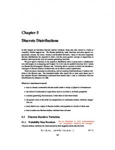
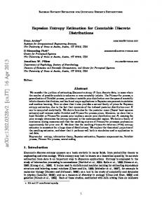
The combined test rejects H0 whenever the min{Pe (n, p0 ), Pa (n, p)} ≤ α. All the above tests are invariant under the transformation X → n − X and the induced transformation p → 1 − p. One of the implications is that the sizes of an invariant test are the same when H0 : p = p0 vs. Ha : p ̸= p0 and when H0 : q = q0 vs. Ha : q ̸= q0 , where q = 1 − p and q0 = 1 − p0 . 3.1.2 Exact Sizes and Powers of the Binomial Tests The sizes and powers of the exact test (6), the alternative test (7) and the combined test are computed using (4) for different parameter and sample size configurations, and plotted them in Figures 1-3. In Figure 1(a − d), we plotted the sizes of the tests as a function of p, and in Figure 2(a − d), we plotted them as a function of n. It is clear from these plots that the sizes of the alternative exact test are closer to the nominal level than are the sizes of the exact test. The sizes of the combined test exceed the nominal level in a few cases but not more than 0.06. Furthermore, the plots of powers in Figure 3(a − d) show that the alternative exact test is not uniformly more powerful than the exact test. But the combined test is either as powerful as the exact test (see Figure 3b and c) or more powerful than the exact test (see Figure 3a and d). 3.1.3 Confidence Intervals for a Binomial Proportion The usual exact confidence limits due to Clopper and Pearson (1934) is given by (beta(α/2; k, n − k + 1), beta(1 − α/2; k + 1, n − k)),

(8)

where beta(c; a, b) denotes the cth quantile of a beta distribution with shape parameters a and b. This interval should be used with the convention that beta(α/2; 0, n + 1) = 0 and beta(1 − α/2; n, 0) = 1. This interval is equivalent to the set {p : P (X ≤ k|p) > α/2} ∪ {p : P (X ≥ k|p) > α/2}, which is the acceptance region of the usual exact test. Because the combined test is better than the usual test, the confidence interval based on the former is shorter than the one based

7 on the latter. Let (pl , pu ) denote the 1 − α confidence interval based on the combined test. Then, min{Pe (n, p), Pa (n, p)} > α for all p ∈ [pl , pu ] and min{Pe (n, p), Pa (n, p)} ≤ α for all p ∈ / [pl , pu ]. Using a searching method with endpoints of (8) as initial values, one can find (pl , pu ). The following algorithm is useful to compute the confidence interval (pl , pu ) for a binomial proportion p. Algorithm 1 For a given k, n and α: Set p = beta(α/2; k, n − k + 1) Set ϵ = 0.001 1 Compute f (n, p) = min{Pa (n, p), Pu (n, p)} If f (n, p) > α then pl = p; goto 2 Else set p = p + ϵ; goto 1 2 Set p = beta(1 − α/2; k + 1, n − k)); 3 Compute f (n, p) = min{Pa (n, p), Pu (n, p)} If f (n, p) > α then pu = p; goto 4 Else set p = p − ϵ; goto 3 4 end We computed the 95% confidence intervals (pl , pu ) using the above algorithm for some values of n and k. These intervals along with the intervals (BS) due to Blyth and Still (1983) are given in Table 2. We observe from the tabulated values that the combined intervals and BS intervals are practically the same except for a few cases. For example, when (n, k) = (8, 0), (9, 0), (11, 0), and (14, 2), BS intervals are slightly shorter than the combined intervals; for (n, k) = (6, 1), (8, 2), (9, 3) and (14, 4), the combined intervals are slightly shorter than the BS intervals. We indeed computed the 95% and 99% combined intervals (not reported here) for all the combinations of (n, k) given in Table 2 of Blyth and Still (1983), and found that the new intervals and the BS intervals are essentially the same for all the cases. Therefore, our combined interval has all the four natural properties listed by Blyth and Still (1983). Furthermore, we observed that our intervals in Table 2 are members of the “complete class” of intervals given in Table 1 of Casella (1986). Remark 1. In a very few situations, the alternate exact method produced disconnected confidence intervals. For example, when n = 13 and k = 0, the alternative method produced (0,.23) and (.260,.269). In this case, the usual exact confidence interval is (0,.23) and hence the combined interval, which is the intersection of the usual exact interval and the alternative exact intervals, is (0,.23).

8 3.2 Poisson Distribution The pmf of a Poisson random variable with mean λ is given by f (x; λ) =

e−λ λx , λ > 0, x = 0, 1, 2, .... x! ∑

Let X1 , ..., Xn be a sample from Poisson(λ). Since Y = ni=1 Xi ∼ Poisson(nλ), testing about λ is equivalent to testing about nλ. Therefore, without loss of generality, we can assume that n = 1. 3.2.1 Hypothesis Tests for a Poisson Mean For an observed value k of Y , the p-value of the usual test for testing H0 : λ = λ0 vs. Ha : λ ̸= λ0 is given by Pe (λ0 ) = 2 min{P (Y ≤ k|λ0 ), P (Y ≥ k|λ0 )}.

(9)

The p-value of the alternative exact test is given by Pa (λ0 ) = P (Y ≤ [λ0 − |k − λ0 |]|p0 ) + P (Y ≥ [λ0 + |k − λ0 |]|p0 ) .

(10)

The combined test rejects H0 whenever the min{Pe (λ0 ), Pa (λ0 )} ≤ α. 3.2.2 Exact Sizes and Powers of the Poisson Tests The sizes and powers of the above Poisson tests are computed using (4), and they are plotted in Figures 4 and 5. The plot in Figure 4a shows that the sizes of the the combined test never exceed the nominal level for λ = 0.5(0.5)60. However, the plot of the sizes for λ = 0.2(0.2)60 in Figure 4b shows that the sizes of the combined test exceed the nominal level at several places but, in general, not more than 0.06. The power plots in Figures 5a and 5b show that the combined test is more powerful than the exact test whereas the alternative exact test is not uniformly better than the exact test. 3.2.3 Confidence Intervals for a Poisson Mean For an observed value k of Y , the classical exact confidence interval for the Poisson mean due to Garwood (1936) is given by (

)

1 1 2 χ2k,α/2 , χ22k+2,1−α/2 , 2 2

(11)

where χ2m,c denotes the cth quantile of the chi-squared distribution with df = m. This interval should be used with the convention that χ20,α/2 = 0. The combined interval is given by {λ : min{Pe (λ), Pa (λ)} > α}.

9 We used a searching algorithm similar to Algorithm 1 with endpoints of (11) as initial values to compute 95% confidence intervals. These combined intervals along with the intervals (CR) due to Casella and Robert (1989) are given for k = 0, 1, ..., 49 in Table 3. It should be noted that the Casella and Robert’s procedure gives a class of intervals for a given k. For example, when k = 12, the right endpoint is any number in the interval 20.77±1.26. The left endpoint of the combined interval and the left endpoint of the CR interval are the same or close whenever the latter is unique (e.g., see k = 0 to 7, 20 and 28 in Table 3). Furthermore, in most cases the combined intervals are members of the class of the CR intervals; in other cases they are very close to the CR intervals (e.g., see k = 21, 26 and 44 in Table 3). 4. Hypergeometric and Negative Binomial Distributions We shall now illustrate the new method for the hypergeometric and negative binomial distributions. 4.1 Hypergeometric Distribution Let X ∼ hypergeometric(N, M, n), where N is the lot size, M is the number of defective items in the lot, and n is the sample size. The pmf of X is given by ( )(

fX (k) =

n k

N −M n−k ( ) N n

)

, max{0, M − N + n} ≤ k ≤ min{n, M }.

Let π = M/N denote the proportion of defective items in the lot. 4.1.1 Hypothesis Tests Consider H0 : π = π0 vs. Ha : π ̸= π0 , where π = M/N . Let M0 = [N π0 ], where [x] denotes the largest integer less than or equal x. For an observed value k of X, we have Pe (M0 ) = 2 min{P (X ≤ k|N, M0 , n), P (X ≥ k|N, M0 , n)}

(12)

and Pa (M0 ) = P (X ≤ [nπ0 − |k − nπ0 |]|N, M0 , n) + P (X ≥ [nπ0 + |k − nπ0 |]|N, M0 , n) . (13) The combined test rejects H0 whenever min{Pe (M0 ), Pa (M0 )} ≤ α. 4.1.2 Confidence Interval for π The left endpoint of the usual exact interval is the value of M for which P (X ≥ k|N, M, n) = α/2 and the right endpoint is the value of M for which P (X ≤ k|N, M, n) = α/2. The confidence set for M based on the combined test is given by {M : min{Pe (M ), Pa (M )} > α}.

10 This set can be obtained using an algorithm similar to Algorithm 1 with ϵ = 1. To get the left endpoint Ml of the confidence interval for M , we used backward search from the integer part of the mean = kN/n. The right endpoint Mu can be obtained using forward search from the mean. We computed 95% confidence intervals for π = M/N based on the usual exact method and the new method, and presented them in Table 4. The values of (n, k) in Table 4 are chosen as in Table 3 for the binomial case so that we can understand the effect of the finite population size in estimating the proportions. We observed from Table 4 that the combined interval is shorter than the usual exact intervals for all the cases. Furthermore, these intervals are shorter than corresponding binomial based intervals which is expected because in the latter case the population is infinite. 4.2 Negative Binomial Distribution In the binomial case the random variable represents the number of successes in n Bernoulli trials whereas in the negative binomial case the random variable represents the number of trials (or the number of failures) required to have a specified number successes. Thus, these two distributions are related, and the results for the negative binomial case can be easily deduced from those of the binomial. The pmf of the negative binomial distribution is given by ( ) k+r−1 r fX (k) = P (X = k) = p (1 − p)k , k = 0, 1, 2, ..., 0 < p < 1, k where X represents the number of failures until the rth success in a sequence of independent Bernoulli trials. 4.2.1 Hypothesis Tests for Negative Binomial p For a given number of failures k until the rth success, the p-value of the usual exact test for testing H0 : p = p0 vs. Ha : p ̸= p0 is given by Pu (r, p0 ) = 2 min{P (X ≤ k|r, p0 ), P (X ≥ k|r, p0 )}.

(14)

Noting that, under H0 , the mean of X is µ0 = r(1 − p0 )/p0 , the p-value of the new test is given by Pa (r, p0 ) = P (X ≤ [µ0 − |µ0 − k|]|r, p0 ) + P (X ≥ [µ0 + |µ0 − k|]|r, p0 ).

(15)

The p-value of the new test is given by min{Pu (r, p0 ), Pa (r, p0 )}. 4.2.2 Confidence Limits for the Negative Binomial p The usual exact limit based on the Clopper-Pearson approach is given by (beta(α/2; r, k + 1), beta(1 − α/2; r, k)). The above limits can be obtained by using the relations among the binomial, negative binomial and beta distributions (e.g., Casella and Berger 2002, p. 454). The confidence interval

11 based on the new test is given by {p : min{Pu (r, p0 ), Pa (r, p0 ) > α}. This interval can be obtained along the lines given for binomial confidence interval. We computed 95% confidence intervals for some selected values of r and k, and presented them in Table 5. It is seen from the table that the left endpoints of the usual interval and the new interval are the same, and the right endpoint of the new interval is less than or equal to that of the usual interval for all the cases considered. 5. Concluding Remarks It should be clear from the preceding sections that the alternative exact test and the usual exact test are the same for testing one-sided hypotheses. For example, in the binomial case, a right-tail test can be used only when k > np0 , and in this case the p-value of the usual test is P (X ≥ k) = P (X ≥ [np0 − |k − np0 |]) which is the p-value of the alternative exact test. Therefore, the alternative test and the usual exact test are the same. This implies that the one-sided limits based on the usual exact method and the combined method are the same. Regarding coverage probabilities of the confidence intervals, we note that the sizes of the new tests for the binomial and Poisson cases never exceeded 0.06, and hence the coverage probabilities for these cases will be at least 0.94 when the confidence level is 0.95. In a recent article, Baker (2000) has noted that the confidence intervals due to Blyth and Still (1983) do not posses nested property; that is, for α′ > α′′ , a 1 − α′ confidence interval may not be a proper subset of a −α′′ confidence interval. As we already pointed out, the proposed tests are simple to use. The p-values of the tests can be computed using available electronic calculators (e.g., TI-83), online calculators (e.g., http://calculators.stat.ucla.edu), and freely available PC calculator StatCalc from http://www.ucs.louisiana.edu/∼kxk4695. For constructing confidence intervals a computer program is necessary, which can be easily written based on our Algorithm 1 for the binomial case. Similar programs can be written for other distributions as well. References Agresti, A. and Coull, B. A. (1998). Approximate is Better than “Exact” for Interval Estimation of Binomial Proportion. The American Statistician 52, 119–125. Blyth, C. R. and Still, H. A. (1983). Binomial Confidence Intervals. Journal of the American Statistical Association 78, 108–116. Brown, L. D., Cai, T. and Das Gupta, A. (2001). Interval Estimation for a Binomial Proportion. Statistical Science 16, 101–133. Burstein, H. (1975). Finite population correction for binomial confidence limits. Journal of the American Statistical Association 70, 67-69. Casella, G. (1986). Refining Poisson Confidence Intervals. The Canadian Journal of Statistics 14, 113–127.

12 Casella, G. and Berger, R. L. (2002). Statistical Inference, Pacific Grove, CA: Duxbury. Casella, G. and Robert, C. (1989). Refining Poisson Confidence Intervals. The Canadian Journal of Statistics 17, 45–57. Clopper, C. J. and Pearson, E. S. (1934). The Use of Confidence or Fiducial Limits Illustrated in the Case of Binomial. Biometrika 26, 404–413. Garwood, F. (1936). Fiducial Limits for the Poisson Distribution. Biometrika 28, 437-442. Krishnamoorthy, K., Thomson, J. and Cai, Y. (2002). An Exact Method of Testing Equality of Several Binomial Proportions to a Specified Standard. To appear in Computational Statistics and Data Analysis. Kulkarni, P. M. and Shah, A. K. (1995). Testing the equality of several binomial proportions to a prespecified standard. Statistics & Probability Letters 25, 213-219.

(a)

(b)

n = 14

0.08 0.07 0.06 0.05 0.04 0.03 0.02 0.01 0

exact alternate combined

0 0.05 0.1 0.15 0.2 0.25 0.3 0.35 0.4 0.45 0.5 p (c)

exact alternate combined

0 0.05 0.1 0.15 0.2 0.25 0.3 0.35 0.4 0.45 0.5 p (d)

n = 25

0.08 0.07 0.06 0.05 0.04 0.03 0.02 0.01 0

n = 17

0.08 0.07 0.06 0.05 0.04 0.03 0.02 0.01 0

n = 33

0.08 0.07 0.06 0.05 0.04 0.03 0.02 0.01 0

exact alternate combined

0 0.05 0.1 0.15 0.2 0.25 0.3 0.35 0.4 0.45 0.5 p

exact alternate combined

0 0.05 0.1 0.15 0.2 0.25 0.3 0.35 0.4 0.45 0.5 p

Figure 1: Sizes of the Tests as a Function of p (a)

(b)

p = 0.1

0.08 0.07 0.06 0.05 0.04 0.03 0.02 0.01 0

exact alternate combined

0

10

20

30 n (c)

40

50

60

10

20

0

10

20

30 n

30 n (d)

40

50

60

13

50

60

exact alternate combined

0

Figure 2: Sizes of the Binomial Tests as a Function of n

40

p = 0.4

0.08 0.07 0.06 0.05 0.04 0.03 0.02 0.01 0

exact alternate combined

0

exact alternate combined

p = 0.3

0.08 0.07 0.06 0.05 0.04 0.03 0.02 0.01 0

p = 0.2

0.08 0.07 0.06 0.05 0.04 0.03 0.02 0.01 0

10

20

30 n

40

50

60

(a)

(b)

n = 13, p0 = 0.1

1

1

exact alternate combined

0.8

n = 13, p0 = 0.25 exact alternate combined

0.8

0.6

0.6

0.4

0.4

0.2

0.2

0

0 0

0.2

0.4

0.6

0.8

1

0

0.2

0.4

p (c)

(d)

1

n = 17, p0 = 0.15

1

exact alternate combined

0.8

0.8

p

n = 20, p0 = 0.25

1

0.6

exact alternate combined

0.8

0.6

0.6

0.4

0.4

0.2

0.2

0

0 0

0.2

0.4

0.6

0.8

1

0

0.2

0.4

p

0.6

0.8

1

p

Figure 3: Powers of the Binomial Tests as a Function of p

0.08 exact alternate combined

0.07 0.06 0.05 0.04 0.03 0.02 0.01 0 0

10

20

30 λ

40

50

Figure 4a: Sizes of the Poisson Tests at α = 0.05; λ = 0.5(0.5)60

14

60

0.08 exact alternate combined

0.07 0.06 0.05 0.04 0.03 0.02 0.01 0 0

10

20

30 λ

40

50

60

Figure 4b: Sizes of the Poisson Tests at α = 0.05; λ = 0.2(0.2)60

(a)

H0 : λ = 5 vs. Ha : λ ̸= 5

1

(b)

1

exact alternate combined

0.8

H0 : λ = 9 vs. Ha : λ ̸= 9 exact alternate combined

0.8

0.6

0.6

0.4

0.4

0.2

0.2

0

0 0

5

10

15

20

25

0

λ

5

10

15 λ

Figure 5: Powers of the Poisson Tests at α = 0.05;

15

20

25

n k 0 1 2 3 n k 0 1 2 3 4 5 n k 0 1 2 3 4 5 6 n k 0 1 2 3 4 5 6 7 8

1 (1) .00 .05

.95 1

5 (1) .00 .01 .08 .19 .34 .50 (1) .00 .01 .04 .10 .17 .25 .32 (1) .00 .00 .03 .07 .11 .17 .22 .26 .34

.50 .66 .81 .92 .99 1 9 .32 .44 .56 .68 .75 .83 .90 13 .23 .34 .43 .52 .59 .66 .74 .78 .83

Table 2: 95% confidence intervals for a binomial proportion (1) Blyth and Still’s (1983) intervals; (2) the combined intervals 2 3 4 (2) (1) (2) (1) (2) (1) .00 .95 .00 .78 .00 .78 .00 .63 .00 .63 .00 .53 .05 1 .03 .97 .03 .97 .02 .86 .02 .86 .01 .75 .22 1 .22 1 .14 .98 .14 .98 .10 .90 .37 1 .37 1 .25 .99 6 7 8 (2) (1) (2) (1) (2) (1) .00 .50 .00 .41 .00 .42 .00 .38 .00 .38 .00 .36 .01 .66 .01 .59 .01 .58 .01 .55 .01 .55 .01 .50 .08 .81 .06 .73 .06 .73 .05 .66 .05 .66 .05 .64 .19 .92 .15 .85 .15 .85 .13 .77 .13 .77 .11 .71 .34 .99 .27 .94 .27 .94 .23 .87 .23 .87 .19 .81 .50 1 .42 .99 .42 .99 .34 .95 .34 .95 .29 .89 10 11 12 (2) (1) (2) (1) (2) (1) .00 .33 .00 .29 .00 .30 .00 .26 .00 .27 .00 .24 .01 .44 .01 .44 .01 .44 .01 .40 .01 .41 .01 .37 .04 .56 .04 .56 .04 .55 .03 .50 .03 .50 .03 .46 .10 .67 .09 .62 .09 .62 .08 .60 .08 .59 .07 .54 .17 .75 .15 .70 .15 .70 .14 .67 .14 .67 .12 .63 .25 .83 .22 .78 .22 .78 .20 .74 .20 .73 .18 .71 .33 .90 .29 .85 .30 .85 .26 .80 .27 .80 .24 .76 14 15 16 (2) (1) (2) (1) (2) (1) .00 .23 .00 .23 .00 .23 .00 .22 .00 .22 .00 .20 .00 .35 .00 .32 .00 .32 .00 .30 .00 .30 .00 .30 .03 .43 .03 .42 .03 .43 .02 .39 .03 .40 .02 .37 .07 .52 .06 .50 .06 .50 .06 .47 .06 .47 .05 .44 .11 .59 .10 .58 .10 .57 .10 .53 .10 .53 .09 .50 .17 .65 .15 .63 .15 .63 .14 .61 .14 .60 .13 .56 .22 .73 .21 .68 .21 .68 .19 .67 .19 .67 .18 .63 .27 .78 .24 .76 .25 .75 .22 .71 .23 .71 .20 .70 .35 .83 .32 .79 .32 .79 .29 .78 .29 .77 .27 .73

16

(2) .00 .01 .10 .25

.53 .75 .90 .99

(2) .00 .01 .05 .11 .19 .29

.37 .50 .63 .71 .81 .89

(2) .00 .01 .03 .07 .12 .18 .25

.25 .37 .46 .54 .63 .71 .75

(2) .00 .00 .02 .05 .09 .13 .18 .22 .27

.21 .30 .37 .44 .50 .56 .63 .69 .73

k 0 1 2 3 4 5 6 7 8 9 10 11 12 13 14 15 16 17 18 19 20 21 22 23 24

Table 3. 95% confidence intervals for a Poisson mean (1) Casella and Robert (1989) intervals; (2) the combined intervals (1) (2) k (1) 0.00 3.54 ± 0.25 0 3.69 25 16.77 36.59 ± 0.55 0.05 5.49 ± 0.16 0.05 5.57 26 16.98 ± 0.21 37.97 ± 0.29 0.36 7.04 ± 0.35 0.36 7.22 27 18.10 ± 0.47 39.03 ± 0.86 0.82 8.56 ± 0.45 0.82 8.77 28 19.05 40.25 ± 1.23 1.37 10.04 ± 0.45 1.37 10.24 29 19.51 ± 0.46 41.48 ± 1.15 1.97 11.51 ± 0.34 1.97 11.67 30 20.77 ± 1.26 42.54 ± 0.79 2.61 12.98 ± 0.16 2.61 13.06 31 21.35 ± 1.17 43.95 ± 0.02 3.28 14.26 ± 1.28 3.29 14.42 32 22.02 ± 0.80 44.99 ± 1.13 3.54 ± 0.25 15.54 ± 0.66 3.98 15.76 33 23.43 46.05 ± 0.77 4.46 16.98 ± 0.21 4.50 17.08 34 23.45 ± 0.02 47.46 ± 0.05 5.32 18.10 ± 0.47 5.32 18.39 35 24.52 ± 0.81 48.49 ± 1.15 5.49 ± 0.16 19.51 ± 0.46 6.00 19.68 36 25.94 49.54 ± 0.80 6.69 20.77 ± 1.26 6.69 20.96 37 25.95 ± 0.01 50.95 ± 0.01 7.04 ± 0.35 22.02 ± 0.80 7.50 22.23 38 27.01 ± 0.88 51.97 ± 1.22 8.11 23.45 ± 0.02 8.10 23.49 39 28.14 ± 0.39 53.03 ± 0.88 8.56 ± 0.45 24.52 ± 0.81 9.00 24.74 40 28.97 54.12 ± 0.42 9.59 25.95 ± 0.01 9.60 25.98 41 29.49 ± 0.52 55.46 ± 0.46 10.04 ± 0.45 27.01 ± 0.88 10.50 27.22 42 30.57 ± 0.56 56.49 ± 1.00 11.18 28.14 ± 0.39 11.18 28.45 43 31.68 57.59 ± 0.58 11.51 ± 0.34 29.49 ± 0.52 12.00 29.67 44 31.97 ± 0.30 58.96 ± 0.23 12.82 30.57 ± 0.56 12.82 30.89 45 33.04 ± 0.76 59.99 ± 1.16 12.98 ± 0.16 31.97 ± 0.30 13.50 32.10 46 34.41 61.04 ± 0.79 14.26 ± 1.28 33.04 ± 0.76 14.50 33.31 47 34.45 ± 0.05 62.25 ± 1.21 14.92 ± 1.07 34.45 ± 0.05 15.00 34.50 48 35.51 ± 0.98 63.47 ± 1.32 15.54 ± 0.66 35.51 ± 0.98 16.00 35.71 49 36.59 ± 0.55 64.51 ± 1.02

17

(2) 16.77 17.50 18.50 19.05 20.00 20.97 21.50 22.50 23.43 24.00 25.00 25.95 26.50 27.50 28.50 29.00 30.00 31.00 31.68 32.50 33.50 34.41 35.00 36.00 37.00

36.90 38.10 39.28 40.47 41.65 42.83 44.00 45.17 46.34 47.50 48.68 49.84 51.00 52.16 53.31 54.47 55.62 56.77 57.92 59.07 60.21 61.36 62.50 63.64 64.78

Table 4. n k 0 1 2 3 4 n k

1 (1) 0 .027

(2) .973 1

0 .053

95% confidence intervals for a hypergeometric π = M/N ; N=150 (1) the usual exact intervals; (2) the combined intervals 2 3 4 (1) (2) (1) (2) (1)

.947 1

0 .013 .167

5 (1)

0 1 2 3 4 n k

0 .007 .060 .153 .293

0 1 2 3 4 5 6 n k

0 .007 .033 .080 .147 .220 .313

0 1 2 3 4 5 6 7 8

0 .007 .027 .060 .100 .153 .207 .267 .333

(1)

0 .013 .080 .200 .353

(1) .500 .647 .800 .920 .987

(2) .327 .467 .587 .687 .780 .853 .920 13

(1)

.773 .973 1

0 .013 .100 .300

0 .007 .047 .107 .180 .260 .333

0 .007 .033 .073 .120 .173 .233 .287 .347

0 .007 .047 .127 .233

.447 .633 .767 .873 .953 10

.327 .440 .553 .667 .740 .820 .893

0 .007 .033 .073 .133 .200 .273 (1)

.227 .340 .420 .500 .573 .653 .713 .767 .827

0 .007 .027 .053 .093 .140 .187 .247 .300

0 .013 .067 .160 .280

(1) .413 .580 .720 .840 .933

(2) .293 .433 .540 .640 .727 .800 .867 14

0 .020 .140 .373

.627 .860 .980 1

0 .007 .073 .200 .407

0 .007 .040 .093 .160 .233 .300

0 .007 .033 .067 .113 .160 .220 .260 .327

0 .007 .040 .107 .193

.400 .567 .700 .807 .893 11

.293 .400 .513 .600 .700 .767 .840

0 .007 .027 .067 .120 .180 .247 (1)

.213 .320 .387 .473 .540 .607 .673 .740 .780

18

0 .007 .020 .053 .087 .127 .173 .227 .280

0 .013 .060 .133 .233

(1) .353 .533 .647 .767 .867

(2) .273 .400 .507 .593 .680 .753 .820 15

0 .013 .107 .253 .480

.520 .747 .893 .987 1

0 .007 .040 .087 .147 .207 .273

0 .007 .033 .067 .107 .153 .200 .240 .300

0 .007 .040 .093 .167

(2) .360 .513 .640 .747 .833 12

(1) .267 .400 .500 .587 .647 .727 .793

(2) .207 .307 .387 .467 .533 .600 .660 .720 .773

.593 .800 .927 .993 1 8

(2)

(1)

(2) .220 .327 .413 .493 .567 .633 .700 .753 .813

.700 .900 .987 1 7

(2)

(1)

(2) .233 .347 .440 .520 .600 .667 .733 .793 .847

0 .027 .227

6 (2)

.513 .707 .847 .940 .993 9

.833 .987 1

(2)

0 .007 .027 .060 .107 .160 .227

0 .007 .020 .047 .080 .120 .167 .213 .260

.360 .500 .620 .700 .800

(2) .253 .373 .467 .560 .640 .707 .773 16

(1) .200 .300 .373 .467 .533 .587 .640 .700 .760

0 .007 .053 .120 .200

0 .007 .033 .080 .133 .193 .253

.247 .373 .453 .540 .620 .687 .747

(2) .193 .287 .367 .440 .507 .573 .627 .687 .740

0 .007 .027 .060 .100 .140 .187 .227 .287

.187 .280 .367 .433 .500 .560 .620 .667 .713

Table 5. r+k r 1 2 3 4 r+k r

1 (1)

(2)

.025

1

.025

(1) 1

95% confidence intervals for a negative binomial p 2 3 (2) (1) (2) (1)

.013 .158

.975 1

5 (1)

1 2 3 4 r+k r

.005 .053 .147 .284

1 2 3 4 5 6 r+k r

.003 .028 .075 .137 .212 .299

1 2 3 4 5 6 7 8

.002 .019 .050 .091 .139 .192 .251 .316

(1)

.005 .053 .147 .284

(1) .527 .751 .902 .987

(2) .369 .527 .651 .755 .843 .915 13

(1)

.003 .028 .075 .137 .212 .299 (2)

.265 .385 .484 .572 .651 .723 .789 .848

.950 1

.008 .094 .292

.842 .987 1

6 (2)

.602 .806 .932 .994 9

.013 .158

.002 .019 .050 .091 .139 .192 .251 .316

.004 .043 .118 .223 (1)

.312 .471 .600 .711 .807 .889

.003 .025 .067 .122 .187 .262 (1)

.221 .002 .339 .018 .438 .047 .527 .084 .609 .128 .685 .177 .755 .230 .819 .289 Note: (1)

.004 .043 .118 .223

(1) .451 .657 .811 .924

(2) .336 .482 .600 .701 .788 .863 14

.776 .975 1

.006 .068 .194 .398

(2) .708 .906 .992 1

7 (2)

.522 .716 .853 .947 10

.008 .094 .292

4

.003 .025 .067 .122 .187 .262

.004 .037 .099 .184 (1)

.283 .429 .550 .655 .749 .831

(2)

.002 .023 .060 .109 .167 .234 (1)

.247 .002 .206 .002 .232 .360 .018 .316 .017 .339 .454 .047 .410 .043 .428 .538 .084 .495 .078 .508 .614 .128 .573 .118 .581 .684 .177 .645 .163 .649 .749 .230 .713 .213 .711 .808 .289 .776 .266 .770 Exact intervals; (2) the combined

19

.004 .037 .099 .184

(1) .393 .582 .729 .847

(2) .308 .445 .556 .652 .738 .813 15

.631 .865 .983 1

8 (2)

.459 .641 .777 .882 11

.006 .068 .194 .398

.002 .023 .060 .109 .168 .234

.003 .032 .085 .157

(2) .410 .579 .710 .816 12

(1) .259 .394 .507 .607 .696 .778

(2) .002 .193 .017 .297 .043 .385 .078 .466 .118 .540 .163 .610 .213 .675 .266 .736 intervals.

.002 .021 .055 .099 .152 .211

.348 .521 .659 .775

(2) .285 .413 .518 .610 .692 .766 16

(1) .002 .016 .040 .073 .110 .152 .198 .247

.003 .032 .085 .157

.002 .021 .055 .099 .152 .211

.238 .364 .470 .564 .650 .729

(2) .218 .319 .405 .481 .551 .616 .677 .734

.002 .016 .040 .073 .110 .152 .198 .247

.181 .279 .363 .440 .511 .577 .640 .700