A simple, intuitive camera calibration tool for natural images. A D Worrall, G D Sullivan and K D Baker Department of Computer Science The University of Reading, Berkshire, RG6 2AY, UK
[email protected] Abstract The paper reports an interactive tool for calibrating a camera, suitable for use in outdoor scenes. The motivation for the tool was the need to obtain an approximate calibration for images taken with no explicit calibration data. Such images are frequently presented to research laboratories, especially in surveillance applications, with a request to demonstrate algorithms. The method decomposes the calibration parameters into intuitively simple components, and relies on the operator interactively adjusting the parameter settings to achieve a visually acceptable agreement between a rectilinear calibration model and his own perception of the scene. Using the tool, we have been able to calibrate images of unknown scenes, taken with unknown cameras, in a matter of minutes. The standard of calibration has proved to be sufficient for model-based pose recovery and tracking of vehicles.
1
Introduction
Any practitioner of 3D vision knows that camera calibration is a time-consuming chore [5]. Many methods for obtaining a description of the 3D structure of a scene depend critically on having an accurate camera model. In the case of a simple pin-hole camera this specifies the 6 extrinsic parameters (the position and orientation of the camera in some world coordinate system) and the 4 intrinsic parameters (the principal point in the image, where the ray through the focus is orthogonal to the image, the focal length of the projection, and the aspect ratio of the discrete sampling of the image). Armed with such information, the small differences between images taken with cameras in different positions can be used to recover the depth of points in the scene, either from multiplecamera stereopsis or from camera movement. Our own work to recover descriptions of traffic scenes using static monocular cameras (e.g. [2]), also relies on camera calibration, but requires considerably less accuracy. The main task in traffic surveillance applications is to recover the pose of rigid objects, such as vehicles, with respect to the camera; this is equivalent to recovering the camera’s 6 extrinsic parameters, referred to a coordinate frame centred on the vehicle. [The image is also, of course, affected by the 4 intrinsic parameters of the camera, but these are usually calibrated before the pose recovery function.] Even the recovery of the 6 extrinsic parameters for a rigid object in unconstrained view is a daunting task. Fortunately, road traffic is strongly constrained:
Figure 1 Typical traffic scene, with parallel road markings identified under normal circumstances all vehicles move in contact with the road surface, and this reduces their freedoms to (x,y) on the road plane, and the rotation angle about the vertical. This “ground-plane constraint” (GPC) enormously simplifies the vehicle pose recovery problem, and the reduction to only one rotation makes quasi-linear methods feasible [4,6]. But to make use of the GPC we must first know the position of the ground-plane with respect to the camera (or equivalently, the position and orientation of the camera in a world coordinate frame (x,y,z) placed at some known point on the road). We have frequently been asked to demonstrate our traffic understanding methods on video tape supplied by potential end-users. These tapes may have been made specially, or might come from existing traffic surveillance cameras, however, they never come with adequate camera calibration data. Figure 1 gives a still from a typical example. Our first problem is to calibrate the camera, so that the position of the ground-plane is modelled with sufficient accuracy for our pose recovery and tracking algorithms. This paper reports an interactive tool we have developed for the task. It relies on decoupling the process into a sequence of simple operations, which are intuitively obvious, even to a naive user. The camera calibration tool has major practical significance. Our previous technique (using traditional methods, discussed below) requires an accurate model of the scene which may take many hours to prepare. Subsequent calibration of the camera then typically takes a highly skilled operator about 30-60 minutes to perform. The new technique relies on the user’s instinctive perception of the scene, and can be done by a novice after minimal training. It requires no explicit scene model and takes a couple of minutes to carry out. It may used in a large number of situations where the position of a camera is required with respect to a planar surface.
2
Camera calibration
The use of the GPC requires the position and orientation of the camera to be known with
respect to a world reference frame. Conventionally, camera calibration is done by fitting a known 3D model of the scene to the image, and solving the resultant set of equations to recover the perspective projection matrix of the imager. In a laboratory setting, this is usually accomplished by use of a specially constructed calibration grid [5]. In our work with natural scenes we have previously built 3D models of the road markings and visible landmarks on building for this purpose [3]. However, traffic scenes are difficult to model without recourse to a detailed survey, which is both expensive and likely to disrupt the traffic flow. We have therefore developed a more qualitative approach to camera calibration, using interactive software tools. This approach is less accurate than can be achieved from a well-surveyed scene, but since it relies on only two arbitrary measurements on the roadway, it is far more applicable in practice. Our interactive method does not determine the principal point, or the pixel aspect ratio. In practice, the former is rarely far from the centre of the image, and the latter is (in principle) obtainable from knowledge of the CCD geometry and the frame-store sampling rates. Small errors in these estimates do not significantly affect our processing, and in practice can be ignored. However, both these parameters are properties of the sensor and the frame-store, so they normally remain constant. If necessary these could be estimated more accurately using a laboratory rig (e.g. by viewing a square target to determine the pixel aspect ratio). Such tests have shown the assumptions to be valid for our cameras. Of the intrinsic parameters, only the focal length then remains to be determined. To recover the extrinsic parameters, we start by identifying two parallel stretches of road markings, from which we can define the vanishing point in the image for all lines parallel to the road, see Figure 1. We then set the focal length to a nominal value, and place on the image of the scene a simulated reference model, comprised of a rectangular grid, with attached normals, whose projection in the image is always constrained to lie between the parallel lines. The distance from the camera to the model is also set to an arbitrary value and the model is scaled so that it fits between the two parallel lines. The operator then uses a slider bar to roll the model about an axis through the vanishing point, until the model appears to be square with respect to the road. Note that to a fair approximation, the visual effect of this rotation is independent of the assumed focal length and distance of the camera from the coordinate frame. The operator’s visual task turns out to be surprisingly simple, since perception is dominated by the frame of reference instinctively recovered from the image of the roadway, and it is fairly easy to identify when the calibration model looks square. Figure 2(a-c) gives an impression of the perceptual task - at this stage the vertical lines should be ignored, since these are affected by the assumed focal length and height. This procedure completely locates the ground-plane, given the initial assumptions of camera focal length and scale. Only the two assumed values now remain to be determined. The tool has a second interactive control which is used to set the focal length. Each time the focal length is changed the previous calculations are repeated, using the vanishing point and the rotation already set. As the focal length is varied, the tilt angle of the ground-plane and the scale factor continuously co-vary, as illustrated in Figure 3. The scale factor and focal length can now be set either by eye, together with knowledge of the camera height above the ground plane or of a single known distance on the ground, or objectively using two measured distances on the ground plane.
(a)
(b)
(c)
(d)
Figure 2 Calibration model rolling -5° (a) through the perceived veridical (b) to +5° (c) about a line through the vanishing point of the road. The final calibration after estimating the scale and focal length is shown in (d). In the first method we manipulate the focal length until the perspective distortion visible in the calibration model (especially the fact that the normals to the base do not look vertical) becomes comparable to that seen in the image. This then leaves the scale factor to be set using knowledge of one absolute measurement. This could be the height of the camera above the ground plane or may be obtained by identifying any one length on the ground-plane, typically by drawing a line across the roadway (perpendicular to the parallels, as indicated by the calibration model), and specifying its real-world dimension by means of a dialogue box. The second, and more accurate, way to estimate the focal length and scale factor uses two measurements of length on the ground-plane. Although these can be taken in arbitrary directions, it is convenient (and more accurate) if these line up with the calibration model. In Figure 2 we use a longitudinal distance given by white line markings, and a lateral distance, given by the lane width; at least in principle, these conform to highway standards and are known in advance. We draw these two lines on the image and real-world dimension the longitudinal line is set by means of a dialogue box. This is then used to compute the scale factor and the apparent length of the second line. The apparent size of the second calibration line is continuously displayed and the user adjusts the focal length until this too is correct. The apparent size is monotonic with the focal length so it would be possible to perform this last step automatically. However, given the interactive nature of the tool, this is superfluous.
Vanishing Point in Image Centre of projection
vanishing direction
Centre of projection
Vanishing Point in Image vanishing direction
ground-plane
ground-plane Camera Height
Apparent size of calibration length
(a)
Camera Height
Apparent size of calibration length
(b)
Figure 3 The interpretation plane of an image line showing short (a) and long (b) focal lengths, and their effects on the apparent tilt of the ground and the apparent length of a calibration line on the ground; here, the camera height has been kept constant. The result is shown in Figure 2(d) where (by way of confirmation) the verticals of the calibration model now seem well-aligned with the lampposts - compare Figure 2(b) and 2(d). The whole process takes a few minutes. It gives a standard of calibration which has proved quite sufficient for our purposes, and has been used successfully for pose recovery and tracking algorithms which rely on knowledge of the ground plane (e.g. [5]). The main benefit of the approach is that interactive camera calibration requires minimal work at the traffic site. It also decouples the camera parameters in a way that is very easy to appreciate - even by a layman. Since the technique can be used by nonspecialist staff after minimal training, it removes a major operational difficulty that stands in the way of practical applications of vision systems for traffic analysis and other surveillance tasks.
3
Performance
Figure 4 illustrates a laboratory scene, used to assess the accuracy of the method. A piece of A3 paper was placed on the ground of our model traffic scene. The camera was calibrated using the long edges to identify the vanishing point, and the lengths of two perpendicular edges to calibrate distance and focal length. Following calibration, a ruler (measuring 485 mm, and just visible on the road on the left in Figure 4) was placed on the ground to appear at a number of positions in the image. The scale tool was then used to measure the apparent size of the ruler in 3D. Our results varied between 480 and 495, and showed no systematic bias from front to back of the scene, indicating very good calibration of the ground-plane with respect to the camera. Any residual error is probably explained by imprecision of identifying the ends of the ruler in the image. The examples described above might be thought particularly favourable to our method for a number of reasons. Firstly, the convergence of the parallel lines is fairly conspicuous, and the vanishing point can be determined accurately. Secondly, the vanishing line is approximately in the direction of the camera tilt, so that the rotation of the calibration model is easy to judge. Finally, the calibration lengths are positioned so that (up to scale) one is most affected by rotation (the lateral) and the other by focal length (the longitudinal).
Figure 4 Laboratory scene (of our model Figure 5 Calibration of a non-ideal view road layout), showing the calibration (see text). model fitted to a piece of A3 paper. Figure 5 shows a view of our road model designed to be less favourable, in which the parallels converge weakly, and lie across the line of camera tilt. The video tape is in the foreground to improve the observer’s perception of scene geometry, which is essential to the method. Removal of the first two supposed advantages proved to cause no difficulty, but the placement of the calibration lines is more important. Two different pairs of calibration lines are illustrated. The first (shown as thicker black lines in Figure 5) are well suited to the task, and yielded the calibration indicated by the model. The second pair of calibration lines (shown dashed) are not useful, since having set the rotation, they covary with variation of the focal length too closely, and thus fail to constrain the calibration of focal length.
4
Discussion
The representation of the camera geometry used in the calibration process is simple and intuitively pleasing. This is a major advantage in an interactive tool, intended to be used by operatives rather than vision scientists. The method exploits the perceptual abilities of the operator to determine a vanishing point, and to set the rotation angle. Two objective measurements then determine the distance and focal length. These parameters interact in a way that is difficult to control, given an arbitrary frame of reference. The simple tricks of constraining the calibration tool to lie between the identified parallels, and of covarying focal length and scale, make the task easy to perform. The tool was initially motivated by the need to calibrate traffic scenes, where long parallel lines are common. It has effectively overcome a problem which recurs every time a new video sequence needs to be considered in our work. The same problem is encountered in many surveillance applications. However, parallel lines are common (or easy to generate) in almost any visual scene, so the tool could have widespread application. The mathematics of the technique is simple, and bear comparison with the method of calibrating a scene from a known rectangle, reported by Haralick [1]. However, in our case, instead of finding two perpendicular pairs of parallel lines to determine the orientation of the plane, we use one pair of parallel lines - known parallels are more common in natural scenes than rectangles, so our method is more useful for surveillance
applications. We then make use of any two linear measurements to recover both the scale and the focal length, whereas Haralick used the known size of the rectangle, and only recovered scale (in fact his closed-form approach to the problem makes it very difficult to consider focal length as a variable). An additional important advantage of our interactive method, is that it becomes very easy to see how effective the calibration is, and to make iterative adjustments accordingly. Methods based on the closed-form computation of parameters, often hide any calibration errors (due, perhaps, to poor data) within the mathematics, in an all-ornone way, and do not admit intelligent, opportunistic intervention.
References [1]
Haralick R M: Determining camera parameters from the perspective projection of a rectangle. Pattern Recognition, Vol 22 (3) pp 225-230, 1989.
[2]
G D Sullivan, Visual interpretation of known objects in constrained scenes, Phil. Trans. Royal Soc. London, Series B: Biol. Sci., vol.337, 1992, pp.361-370.
[3]
T N Tan, Sullivan, G D and Baker K D. On Computing the perspective transformation matrix and camera parameters. British Machine Vision Conference 1993 pp 125-134.
[4]
T N Tan, G D Sullivan & K D Baker, Recognising objects on the ground plane. Image and Vision Computing, 12:3 pp 164-172 (1994)
[5]
T N Tan, G D Sullivan & K D Baker, Fast vehicle localisation and recognition without line extraction and matching. British Machine Vision Conference 1994 (this volume)
[6]
R Y Tsai Synopsis of recent progress on camera calibration for 3D machine vision in The Robotics Review. O Khatib, et al (Eds) MIT Press, 1989.
[7]
A D Worrall, Sullivan G D and Baker K D. Advances in Model based Traffic Vision. British Machine Vision Conference 1993 pp 559-568
Appendix: Geometrical analysis We define the camera coordinate system with the origin at the centre of projection, and x horizontal, z vertical and y perpendicular to the image plane. The image plane is some distance f (the focal length) in front of the centre of projection. Our task is to construct a new coordinate system whose x-y plane corresponds to the ground plane. We identify two lines in the image which correspond to parallel lines on the ground plane. The vanishing point in the image is given by the row vector: Vd = uv f vv Because of our choice of the camera coordinate system this also defines the vanishing direction. The two parallel lines lie in the ground-plane which must therefore contain the
Vanishing Point in the Image Vanishing Direction Gz
Gy
Centre of Projection
Go
Gx
Ground plane
Figure 6 The interpretation plane of one of the vanishing lines. The ground plane coordinate system is constructed so that Gy is in the vanishing direction, Gx and Gy are in the ground plane, and the origin is on the ray through the centre of the line. vanishing direction. Consider an arbitrary point on the image (for example the midpoint of the left-hand line segments used to define the parallel lines), given by: o = uo f vo We use this as the origin of a set of coordinates on the ground plane, which is at some as yet unknown distance s along the ray defined by o i.e. G o = so = su o sf sv o The coordinate frame on the ground plane is defined by orthogonal axes G x , G y and G z . We choose G y to correspond to the vanishing direction with G x in the ground plane, and hence G z is normal to the ground plane. We obtain these directions by considering two rotation matrices, the first of which takes the camera y-axis into the vanishing direction. The general form for a rotation of angle θ about a arbitrary axis defined by the direction cosines h , k and l is given by1 2
h (1 – cos θ) + cos θ hk(1 – cos θ) + l sin θ hl(1 – cos θ) – k sin θ 2
hk(1 – cos θ) – l sin θ k (1 – cos θ) + cos θ kl(1 – cos θ) + h sin θ hl(1 – cos θ) + k sin θ kl(1 – cos θ) – h sin θ
2
l (1 – cos θ) + cos θ
In our case θ is defined by the inner product between the camera y-axis and the vanishing direction cos θ = yˆ ⋅ vˆ where vˆ is the normalised vanishing direction. The direction cosines are thus determined 1. Transformations are represented by left acting matrices.
by the normalised outer product between the y-axis and the vanishing direction. yˆ ∧ vˆ h k l = -------------yˆ ∧ vˆ hence vz h = --------------------2 2 vx + vz
–vx l = --------------------2 2 vx + vz
k = 0
cos θ = v y
also 2
2
vx + vz =
2
1 – v y = sin θ
Therefore the rotation matrix becomes 2
1 – αv x – v x – αv x v z vx
vy
– αv x v z – v z1
vz 2
– αv z
where 1 – vy 1 α = -------------- = -------------2 1 + vy 1 – vy We still have freedom to rotate the coordinate frame about vanishing direction. This second rotation can be represented by the matrix cos ϕ 0 – sin ϕ 0 1 0 sin ϕ 0 cos ϕ where ϕ = 0 corresponds to the (arbitrary) direction of Gx due to the first rotation. The angle ϕ is determined by user interaction (see Figure 2 of main text). The transformation matrix then becomes 2 1 – αv x cos ϕ + αv x v z sin ϕ vx
v z sin ϕ – v x cos ϕ
2 –1 – αv z sin ϕ – αv x v z cos ϕ
vy
vz
2 2 1 – αv x sin ϕ – αv x v z cos ϕ – v x sin ϕ – v z cos ϕ 1 – αv z cos ϕ – αv x v z sin ϕ
The rows of this matrix are the required axes G x , G y and G z . The top row is the G x -axis in the ground plane
Gx =
2 1 – αv x cos ϕ + αv x v z sin ϕ v z sin ϕ – v x cos ϕ 2 – 1 – αv z sin ϕ – αv x v z cos ϕ
T
The middle row is the G y -axis, the vanishing direction as constructed. Finally the bottom row is the G z -axis normal to the ground plane. 2 1 – αv x sin ϕ – αv x v z cos ϕ Gz = – v x sin ϕ – v z cos ϕ
T
2 1 – αv z cos ϕ – αv x v z sin ϕ
Having defined the ground plane it is straightforward to map any point on the image p to an equivalent point on the ground plane P by considering the intercept of the ray with the ground plane given by the equations P = λp and P ⋅ Gz = Go ⋅ Gz solving for λ we get Go ⋅ Gz λ = ----------------p ⋅ Gz If p is a point on the second of the lines used to define the vanishing point then we can compute the separation of the parallel lines on the ground plane as Go ⋅ Gz G o – -----------------p ⋅ Gx p ⋅ Gz which is linearly dependent on the unknown scale factor s . This distance is used to scale the calibration model so it fits between the parallel lines (see Figure 2). Alternatively, the height of the camera above the ground plane is given by G o ⋅ G z which is also linearly proportional to the unknown scale, so if the camera height is known, the scale can be determined for a given focal length. It is usually easier to arrange that some length on the ground-plane is known, and this too can be used to determine the scale factor. The two end points are marked on the image and are then projected onto the ground-plane with an assumed scale of 1 as above. This corresponds to the physically impossible, but mathematically useful, situation of the ground plane intercepting the image plane at the point o . The scale is then determined by the ratio of the apparent length and the user supplied measurement. d real s = ---------d app Thus for an assumed focal length, the ground plane is completely determined, and the absolute position of any point on the computed ground plane is easy to compute.