Furthermore, it also allows accounting for ... information system (GIS) is also proposed and found to be simple and easy-to- use. ..... Software, 23, 1013-1025. ii.
www.ijird.com
February, 2016
Vol 5 Issue 3
ISSN 2278 – 0211 (Online)
A Simple Lag Time Based GIUH Model for Direct Runoff Hydrograph Estimation S. S. Rawat Scientist, Western Himalayan Regional Centre, National Institute of Hydrology, Jammu & Kashmir, India P. Kumar Scientist, Western Himalayan Regional Centre, National Institute of Hydrology, Jammu & Kashmir, India M. K. Jain Associate Professor, Department of Hydrology, Indian Institute of Technology Roorkee, Uttarakhand, India S. K. Mishra Professor, Department of Water Resources Development and Management, Indian Institute of Technology Roorkee, Uttarakhand, India B. Nikam Scientist, Indian Institute of Remote Sensing, ISRO, Dehradun, Uttarakhand, India Abstract: In this study, direct runoff hydrograph (DRH) is derived by defining the Nash GIUH parameters in terms of the lag time of the watershed, rather than velocity used in conventional GIUH approach. The proposed approach is tested for its applicability on several isolated rainfall-runoff events of a Himalayan watershed (Gagas watershed within Ramganga basin) located in Uttarakhand state of India. The DRHs derived by the proposed approach were found to be in good agreement (average Nash and Sutcliffe Efficiency (NSE) = 83.2% and relative error (RE) in peak = 5.4%) with the observed DRHs. The proposed approach was also compared with kinematic wave-based GIUH approach and the results of the former approach were found superior to the later. Furthermore, to overcome the complexity involved in manual estimation of geomorphological parameters, an approach based on Melton number and geomorphological information system (GIS) is also proposed and found to be simple and easy-touse. Keywords: GIS, GIUH, ILWIS, Lag Time, Nash Model, SRTM DEM.
1. Introduction Linking of hydrological response of a catchment with the geomorphologic characteristics has been of paramount interest to researchers since last three decades. The Instantaneous Unit Hydrograph (IUH) proposed by Rodriguez-Iturbe et al. (1979) and further refined by Gupta et al. (1980), known as geomorphologic IUH (or GIUH) became more promising for ungauged catchments or data deficient catchments. Since the theory incorporates peak discharge (qp) and time to peak (tp) in terms of geomorphological characteristics of river basin, the requirement of land use and climatic parameters is obviously omitted and it is one of its major advantages. Major drawback, however, is that it does not give the complete shape of IUH, and therefore, inheres subjectivity in drawing of the complete hydrograph. Consequently, Rosso (1984) expressed ‘n’ and ‘k’ in terms of Horton ratio and a dynamic velocity parameter using power regression. A number of researchers have investigated the intermittency between hydrological behavior of the catchment and its geomorphology eg; Bhaskar et al. (1997), Hall et al. (2001), Jain et al. (2003), Nasri et al. (2004), Kumar et al. (2007), and Bharda et al. (2008). The major advantage of GIUH theory is that it transforms the net rainfall to runoff by using a transfer function based on the spatial organization of the catchment geomorphology. Furthermore, it also allows accounting for the modification in the drainage system after major runoff events, and thus, the new drainage pattern can be mapped and the geomorphological transfer function can be updated (Nasri at al., 2004). Moreover, the difficulty with GIUH theory is its dependency on a dynamic parameter i.e. velocity. Rodriguez-Iturbe and Valdes (1979) used a constant velocity corresponding to peak discharge considering the flows in watershed occurred at peak discharge velocity. However, the question of how the velocity at peak flow is calculated was not addressed. To circumvent the problem, Rodriguez-Iturbe et al. (1982) related the velocity with the effective rainfall intensity and duration. To investigate the velocity – rainfall-excess functionality, Moughamian et al. (1987) computed GIUH proposed by Rodriguez-Iturbe et al. (1982) and found it to
INTERNATIONAL JOURNAL OF INNOVATIVE RESEARCH & DEVELOPMENT
Page 197
www.ijird.com
February, 2016
Vol 5 Issue 3
perform poorly despite considering the distribution of rainfall-excess derived from sophisticated time varying infiltration capacity methods. Further, Bhaskar et al. (1997) found that the use of rainfall-excess intensity to estimate flow velocity may lead to inaccurate estimation of GIUH qp and tp. Generally, the flow velocity is overestimated by the rainfall-excess intensity approach, which yields smaller value of k and finally yields higher qp and corresponding lower tp. Manual estimation of geomorphologic parameters is a tedious and cumbersome process and often discourages field engineers for developing regional methodologies to solve various hydrological problems of the ungauged catchments or in limited data situations. With advancement in Geographical Information System (GIS) and Remote Sensing (RS), the automated watershed delineation and drainage network extraction from Digital Elevation Model (DEM) has gained much impetus in hydrology since last two decades (Moore et al., 1992; Maathuis, 2005; Hengl et al., 2006). However, the density of drainage network derived using GIS depends on the user-supplied values of drainage network parameters i.e., stream threshold area and minimum source drainage length which involves the subjectivity in extraction. In this context, the present study is carried out to (i) propose a simple and more versatile GIUH approach for Direct Runoff Hydrograph (DRH) estimation, (ii) extract more realistic drainage network from SRTM DEM using a raster based GIS incorporating Melton number concept, and (iii) check the accuracy of the proposed model by comparing observed and estimated DRHs for a Himalayan watershed from Indian subcontinent. 2. Proposed LAG Time Based GIUH Model Nash (1957) proposed an IUH in the form of the two-parameter gamma distribution. The catchment was assumed to be made up of a series of ‘n’ identical linear reservoirs having the same storage coefficient ‘k’. The first reservoir receives a unit volume of effective rainfall instantaneously and it is routed through the first reservoir to the outlet by assuming that the outflow from a reservoir acts as inflow for the next. The Nash IUH can be expressed as:
1 t q (t ) = kΓn k
n −1
t exp − k
(1) where ‘t’ is in hours and q(t) has the dimensions of hour-1. For estimation of ‘n’ and ‘k’, Nash used the first and second order moments of rainfall hyetograph and direct runoff hydrograph, i.e. fully gauged conditions. The following relationships for ‘tp’ (or mode of gamma function) and lag time ‘tl’ (or the first moment of gamma function) are valid for Gamma IUH:
t p = (n − 1)k
(2)
t l = nk
(3) Eqs. (2) and (3) yield tp= tl (n-1)/n, indicating that tp < tl, which is one of the essential conditions of IUH. Substituting ‘tp’ (Eq. 2) into Eq. (1) results into
qp =
1 (n - 1)(n -1) e -(n-1) kΓ n
(4)
Defining a dimensionless term β (= qptp),
β = qpt p =
(n − 1) n −1 e − (n −1) Γ(n − 1)
(5) To link the IUH’s ‘qp’ and ‘tp’ with the catchment geomorphological parameters, Rodriguez-Iturbe and Valdes (1979) related them with dynamic velocity ‘v’ and expressed as:
qp = i v
(6)
t p = k 1 /v
(7)
where ‘i’ and ‘k1’ are expressed respectively as:
1.31 0.43 i= R L L
k1 = 0.44 L R B
0.55
(8)
RA
−0.55
RL
−0.38
(9) where ‘L’ is the length of main channel or length of highest order stream in kilometers, ‘v’ is the average peak flow velocity or characteristic velocity in meter/second, ‘qp’, and ‘tp’ are in units of hr-1 and hr, respectively. Bifurcation ratio ‘RB’, area ratio ‘RA’, and length ratio ‘RL’, expressed as:
A w A w −1 = R A N w N w +1 = R B ; and L w L w −1 = R L . N is the number of streams of order w ;
‘w’; Aw is the mean area of basin of order w; and Lw is the mean length of stream of order ‘w’. A substitution of i (Eq. 8) and k1 (Eq. 9) into (6) and (7), respectively, yields:
INTERNATIONAL JOURNAL OF INNOVATIVE RESEARCH & DEVELOPMENT
Page 198
www.ijird.com
February, 2016
1.31 0.43 qp = R L v L L 0.55 −0.55 −0.38 t p = 0.44 R B R A R L v
Vol 5 Issue 3
(10)
(11) Eqs. (10) and (11) were further re-arranged by Rosso (1984), in which ‘qp’, ‘tP’, ‘L’, and ‘v’ are measured in coherent units, and expressed, respectively, as:
q p = 0.364R L
0.43
R t p = 1.584 B RA
vL−1
(12)
0.55
RL
− 0.38
v −1L (13)
Further, the β can be expressed as:
R β = 0.584 B RA
0.55
RL
0.05
(14) Notably, the expressions derived by Rodriguez-Iturbe and Valdes (1979) assume a triangular IUH and only specify the expressions for ‘qp’ (Eq. 10) and, ‘tP’ (Eq. 11), and therefore, it is very difficult and subjective to draw the complete shape of IUH using only two salient points, qp and tp. To overcome, Rosso (1984) equated both the expressions of non-dimensional term β of GIUH (Eq. 14) and Gamma IUH (Eq. 5) and used an iterative computing scheme to derive the Nash parameters as:
n = 3.29(R B /R A ) 0.78 R L
0.07
(15)
k = 0.70[R A /(R B R L )]0.48 v −1L
(16) Remarkably, the dynamic velocity ‘v’ can vary from storm to storm and even within a storm (Rodriguez-Iturbe and Valdes, 1979), for it involves several parameters like channel slope, Manning roughness coefficient, velocity at different depths, geometric properties of cross-section at gauging site. Hence, the observed value of ‘v’ is rarely available, leading to adoption of an approximate value only, which often leads to severe error. Equating Eq. (5) with Eq. (14), one gets
R (n − 1) n −1 e −(n −1) = 0.584 B Γ(n − 1) RA
0.55
RL
0.05
(17) All the terms in the right hand side of Eq. (17) are known. The only unknown term in Eq. (17) is the Nash model parameter ‘n’, which can be obtained by solving it using a suitable optimization scheme such as Newton-Raphson method. The following text derives ‘v’ from geomorphological and hydrological characteristics of the watershed. Coupling Eqs. (2) and (3) and equating the tp (Eq. 13), one gets
R n − 1 t l = 1.584 B n RA
0.55
RL
−0.38
v −1L (18)
From Eq. (18), velocity ‘v’ can be easily expressed as:
R v = 1.584 B RA
0.55
RL
−0.38
n L n −1 tl
(19)
Finally, substituting ‘v’ (Eq. 19) into Eq. (16), one gets a new expression for k as: 1.03
R k = 0.442 A RB
n −1 (R L ) −0.10 t l n
(20) Notably, the above expressions (Eqs. 17 and 20) do not contain velocity term, and thus, ‘n’ and ‘k’ can be computed from known RA, RB, RL, and tl, parameters using Eqs. (17) and (20), respectively. 2.1. Derivation of Direct Runoff Hydrograph Once ‘n’ and ‘k’ are estimated, the complete shape of GIUH can be derived using Eq. (1), and subsequently, the D-hour UH can be computed as follows:
INTERNATIONAL JOURNAL OF INNOVATIVE RESEARCH & DEVELOPMENT
Page 199
www.ijird.com (D − hour UH) =
February, 2016
Vol 5 Issue 3
1 [(IUH) t + (IUH) t −D ] 2
(21) If two IUHs are lagged by D-hour, where D is small, and their corresponding ordinates are summed up and divided by two, the resulting hydrograph will be a D-hour UH. Finally, DRH can be computed by convolution. 3. Application 3.1. Study Area and Data Used The Gagas watershed is one of the sub-watershed of the Ramganga catchment located in the Himalayan region of India having an area of 506 km2 and lies between latitudes 290 35’ 20” N and 290 51’N and longitudes 790 15’E and 790 35’ 30” E as shown in Fig. 1. Worth notable that Gagas watershed is hydrologically important sub-watershed of Ramganga reservoir catchment (area = 3134 sq. km). Ramganga reservoir which is a multipurpose 127-meter-high earth and rock-fill dam of Government of Uttar Pradesh (India) was built in 1974. It produces approximately 452 million units of electricity annually and also facilitates irrigation in an area of about 5.12 lakh hectare during non-monsoon period. The watershed area in general has a hilly terrain with undulating and irregular slopes (elevation ranging from 772 m to 2744 m from msl) ranging from relatively flat in narrow river valley to steep towards ridge. The mean annual rainfall varies from 903 mm to 1281 mm with a mean value of 1067 mm (Kumar and Kumar, 2008).
Figure 1: Location of study area and drainage networks showing different stream order of Gagas watershed extracted from SRTM-DEM using Melton number concept. The hydrologic data of storm rainfall-runoff for eight isolated single peaked storms were obtained from the Divisional Forest Office, Ranikhet, Uttarakhand, India, and used in this study. Shuttle Radar Topography Mission-Digital Elevation Model (SRTM-DEM) having fineness of 3-arc second spatial resolution (≈90m) were downloaded from Global Land Cover Facility (GLCF, 2008) and used for computation of geomorphological parameters. 3.2. Extraction of Drainage Network A PC-based GIS and Remote Sensing software: Integrated Land and Water Information System (ILWIS) 3.31 have been used to delineate watershed boundary and extract geomorphological parameters for the study watersheds. To delineate the drainage network of the Gagas watershed, the SRTM mosaic DEM was passed through several processes like fill sinks, flow direction, flow
INTERNATIONAL JOURNAL OF INNOVATIVE RESEARCH & DEVELOPMENT
Page 200
www.ijird.com
February, 2016
Vol 5 Issue 3
accumulation, drainage network extraction, drainage network ordering, catchment extraction, and finally, catchment merged according to the location of outlet of the watershed. However, to schematize and parameterize a more realistic drainage network, an adequate value of stream threshold (minimum number of pixels that should drain into a pixel examined to add this pixel to the output drainage map) and minimum drainage length are provided, which fully depend on the user’s familiarity with the study area. However, to examine the most appropriate stream threshold as required by the GIS software, Melton (1958) number approach is employed. Melton number is defined as the stream frequency (stream number per unit area) divided by the square of the drainage density (stream length per unit area). This constant, in fact, relates all the planimetric characteristics of the river network structure, and universally, it can be assumed to have a value of about 0.694 irrespective of the basin scale (Melton, 1958). An approximation to the Melton number was also given by Elsheikh and Gurceio (1997) in terms of Horton ratios as equal to (RB-RL)/(RB-1). To obtain realistic drainage maps of the study areas from the raster DEM, the drainage network was extracted for different stream thresholds (ranging from 1 to 300 pixels) by following the procedure described earlier using ILWIS 3.31 and the corresponding Horton ratios RB, RL, and RA were computed graphically by plotting total number of streams, mean stream length, mean stream area versus order of channel, and slope of lines. Melton numbers were computed using Horton’s ratios for different stream thresholds ranging from 1 pixel to 300 pixels. At threshold value of 60, the Melton number was found 0.662, closest to the aforementioned value (0.694). The geomorphological parameters derived from drainage network (at stream threshold of 60) are given in Table 1. It can be observed from Table 1that the values of RB, RL, and RA are 4.81, 2.29, and 5.45, respectively, for the study watershed. Thus, it can be inferred that RB, RL and RA are within the range as suggested by Rodriguez-Iturbe and Valdes (1979) as: 2.5 ≤ R B ≤ 5.0 ,
3.0 ≤ R A ≤ 6.0 , and 1.5 ≤ R L ≤ 4.0 .These values are very close to the corresponding values, viz. R = 4.82, R = 2.39 and R = B L A 5.37 derived by Kumar and Kumar (2008) from the Survey of India (SOI) topo sheets (Table 1). Total Mean stream Mean stream Bifurcation ratio Stream length Stream Area Number length (km) area (km2) (RB) ratio (RL) ratio (RA) of streams 123 2.19 2.8 25 3.66 17.45 4.81(4.82) 2.29 (2.39) 5.45 (5.37) 7 5.92 68.76 1 29.42 506 Table 1: Geomorphological characteristics of Gagas watershed extracted from SRTM DEM using ILWIS3.31 Note: the values in parenthesis represent corresponding values extracted from SOI topo sheets
Stream Order 1 2 3 4
3.3. Computation of Lag Time (tl) In this study, the approach of distribution hydrograph (Benard, 1935), which is basically a unit hydrograph whose ordinates are expressed in percentage of the surface runoff occurring in successive periods of equal time interval, has been used for tl computation. Distribution hydrograph of Gagas watershed were derived using one of the available storm runoff event of Gagas watershed, for determination of cumulative percentage distribution graphs and, in turn, determine lag time (tl) corresponding to 50% runoff volume as shown in Fig. 2. It can be seen from Fig. 2 that 50% of the runoff volume is passed away within 2 hours. Therefore, the lag time of Gagas watershed is adjudged as 2 hours. Here, it is worth emphasizing that tl is taken as constant consider that peak flow hours of appreciable magnitude are characterized by a relatively small variability of lag time (Boyd, 1982).
Figure 2: Cumulative distributed hydrograph for Gagas Watershed for estimation of lag time.
INTERNATIONAL JOURNAL OF INNOVATIVE RESEARCH & DEVELOPMENT
Page 201
www.ijird.com
February, 2016
Vol 5 Issue 3
4. Results and Discussions The model is tested for its performance on six isolated storm events for which peak discharge vary from 59.2 m3/s to 122 m3/s of Gagas watershed. The model performance is evaluated using Root mean absolute error (RMAE), root mean square error (RMSE), relative error in peak (REP) and Nash-Sutcliffe coefficient of efficiency (NSE). These statistical indices are frequently used in hydrological modeling and easily available in any text book of statistics. Using Eqs. (17) and (20), the parameters ‘n’ and ‘k’ were computed and substituted into Eq. (1) for deriving the complete shape of GIUH. Subsequently, using Eq. (23), the corresponding one-hour UH was derived. Finally, convoluting the unit hydrograph with the rainfall-excess of six storm events, DRHs were predicted as shown in Fig. 3 for different storm events. From these figures, it can be seen that there is a close match between observed and predicted DRHs using lag time GIUH method, especially for time to peak, time base, peak discharge rate and overall shape. The peak discharge is closely predicted by the proposed lag time (LT) method as compare to KW based GIUH method. Table 2 summarizes the statistical errors in estimation of DRHs for different storm events using GIUH approach based on kinematic-wave (KW) theory (Kumar & Kumar 2008) and lag time (LT) based for Gagas watershed. It is seen that both the methods produce almost the same average NSE, RMSE, and RMAE values. However, average peak error due to LT based GIUH method is 5.4% whereas it is 15.2% due to KW based GIUH method. Application of both the methods yield sudden jump in the rising limb of all events which resulted in high RMSE. However, the recession limbs computed by both the methods closely match the observed, but slightly better by KW method. Overall, peak discharge and time to peak being two important characteristics of UH theory, the simple LT method GIUH approach is seen to have performed superior to KW based GIUH approach in this study. It is notable that the prediction accuracy of KW based GIUH approach depends primarily on the degree of accuracy in adoption of Manning’s roughness coefficient for overland and channel flows and these are very sensitive to peak discharge rate and time to peak of IUH, and therefore, the resulting complete shape of GIUH or DRH is quite sensitive. High value of average NSE (83.2%) and low value of average REP (5.4%) also supports the suitability and efficacy of the proposed simple LT based GIUH approach for DRH prediction. The lag time being a fingerprint of the drainage basin, reflecting the storage and velocity of water in its travel over the basin and down channel, is a better index of watershed’s hydrological behavior than the velocity of flow only. Any disturbance in the basin surface and its channels will alter lag time. Thus, lag time based GIUH approach is more versatile than velocity of flow in such endeavors and simpler in general. REP (%) NSE (%) RMSE (m3/s) LT KW LT KW LT KW LT KW June 4, 1977 0.054 0.063 11.364 13.215 1.2 17.3 88.4 84.4 June 25, 1978 0.076 0.065 14.882 14.875 11.7 8.7 85.6 85.6 July 31, 1982 0.068 0.069 6.631 7.239 0.6 18.8 86.3 83.7 August 11, 1983 0.068 0.072 7.900 8.718 4.2 21.7 86.2 83.1 August 10, 1985 0.106 0.075 13.289 11.793 10.4 9.8 69.1 75.6 August 15, 1985 0.073 0.057 10.054 9.886 4.2 14.9 83.7 84.3 Average 0.067 0.074 10.954 10.687 5.4 15.2 83.2 82.8 Table 2: Storm-wise statistical measures for prediction of DRHs using proposed Lag Time (LT) and Kinematic Wave-based (KW) (Kumar and Kumar, 2008) GIUH approaches for Gagas watershed. Storm Date
RMAE
INTERNATIONAL JOURNAL OF INNOVATIVE RESEARCH & DEVELOPMENT
Page 202
www.ijird.com
February, 2016
Vol 5 Issue 3
Figure 3: Comparison between Direct Runoff Hydrograph (DRH) predicted by lag time (LT) and Kinematic-Wave (KW) based GIUH approach with observed DRHs for storm events on: (a) June 4, 1977; (b) June 25, 1978; (c) July 31, 1982; (d) August 11, 1983; (e) August 10, 1985 and (f) August 15, 1985. 5. Conclusion The following conclusions can be derived from this study: 1. A simple GIUH based approach is proposed for derivation of direct runoff hydrographs by defining the Nash gamma IUH parameters ‘n’ and ‘k’ in terms of geomorphological parameters and lag time of the watershed. It is more conceivable than the conventional one due to elimination of dynamic velocity ‘v’, which involves greater subjectivity in its estimation in routine applications. 2. The proposed approach is tested on several storm events of wide range of peak discharge from two Himalayan watersheds and found to perform well, even better than the sophisticated kinematic wave based GIUH approach. 3. A PC-based GIS and Remote Sensing software “Integrated Land and Water Information System (ILWIS)” has been used for extraction of geomorphological parameters from SRTM data for extraction of DEM, drainage network and geomorphological parameters. Melton number concept was used for extraction of realistic drainage network using a GIS software. The suggested methodology might be of help even when topo sheets of the study area are not available. Since geomorphological parameters used in the study were extracted from the easily and freely available SRTM data in GIS environment, the model is easy-to-use for any catchment. 6. References i. Bharda A. Panigrahi, N., Singh, R., Raghuwanshi, N. S., Mal, B. C., and Tripathi, M. P. (2008). Development of geomorphological instantaneous unit hydrograph model for scantly gauged watersheds. Environmental Modelling & Software, 23, 1013-1025. ii. Bhaskar, N. R., Parida, B. P. & Nayak, A. K. (1997). Flood estimation for ungauged catchments using the GIUH. J. Water Resource Plan. Manage. ASCE 123(4), 228–238. iii. Hall, M.J., Zaki, A.F., Shahin, M.M.A., (2001). Regional analysis using the geomorphoclimatic instantaneous unit hydrograph. Hydrol. Earth Sys. Sci. 5(1), 93-102.
INTERNATIONAL JOURNAL OF INNOVATIVE RESEARCH & DEVELOPMENT
Page 203
www.ijird.com
February, 2016
Vol 5 Issue 3
iv. Hengl, T., et al. 2006. Chapter 3: Terrain parameterization in ILWIS. New terrain arameterization text book. (ed.),European Commission Joint Research Centre: 29-48. v. Jain, V. and Sinha, R. (2003). Derivation of unit hydrograph from GIUH analysis for the Himalayan river. Water Resour. Manage., 17, 355–375. vi. Kumar R., Chatterjee, C., Singh, R. D., Lohani, A. K., and Kumar, S. (2007). Runoff estimation for an ungauged catchment using geomorphological instantaneous unit hydrograph (GIUH) model. Hydrol. Process., 21, 1829-1840. vii. Kumar, A., and Kumar, D. (2008). Predicting Direct Runoff from Hilly Watershed Using Geomorphology and Stream-OrderLaw Ratos: case study, J. Hydrologic Engineering, 13(7), 570-576. viii. Maathuis, B. and K. Sijmons (2005). DEM from Active Sensors – Shuttle Radar Topographic Mission (SRTM), International Institute for Geo-Information Science and Earth Observation. ix. Melton, M. A. (1958). Geometric properties of mature drainage systems and their representation in an E4 phase space. J. Geol. 66, 35-54. x. Moore, I. R., et al. (1992). Digital terrain modelling: A review of Hydrological, Geomorphological and Biological applications. Terrain analysis and distributed modelling in hydrology. (ed.) K. Beven and I. R. Moore, John Wiley and Sons: 7-34. xi. Moughamiam, M.S., McLaughlin, D.B., and Bras, R.E. (1987). Estimation of Flood Frequency: An evaluation of two derived distribution procedure. Water resources research, 23, 1309-1319 xii. Nash, J. E. (1959). Synthetic determination of unit hydrograph parameters. J. Geophys. Res. 64(1), 111–115. xiii. Nasri, S., Cudennec, C., Albergel, J. & Berndtsson, R. (2004). Use of geomorphological transfer function to model design floods in small hill side catchments in semi arid Tunisia. J. Hydrol. 287, 197–213. xiv. Rodriguez-Iturbe, I., and J. B. Valde´s (1979), The geomorphologic structure of the hydrologic response, Water Resour. Res., 15(6), 1409– 1420. xv. Rodriguez-Iturbe, I., Gonzalez-Sanabria, M. & Bras, R. L. (1982). The geomorphoclimatic theory of the instantaneous unit hydrograph, Water Resour. Res. 18(4), 877–886. xvi. Rosso, R. (1984). Nash model relation to Horton order ratios, Water Resour. Res., 20(7), 914– 920.
INTERNATIONAL JOURNAL OF INNOVATIVE RESEARCH & DEVELOPMENT
Page 204