A Simple Method for Variable Selection in Regression with Respect to ...

A Simple Method for Variable Selection in Regression with Respect to Treatment Selection Lacey Gunter

Gunter Statistical Consulting Provo, UT 84604 USA [email protected]

Michael Chernick

Director of Biostatistical Services Lankenau Institute for Medical Research Wynnewood, PA 19096 USA

[email protected] Jiajing Sun

Management School The University of Liverpool Liverpool L69 7ZH United Kingdom

[email protected] Abstract In this paper, we compare the method of Gunter et al. (2011) for variable selection in treatment comparison analysis (an approach to regression analysis where treatment-covariate interactions are deemed important) with a simple stepwise selection method that we introduce. The stepwise method has several advantages, most notably its generalization to regression models that are not necessarily linear, its simplicity and its intuitive nature. We show that the new simple method works surprisingly well compared to the more complex method when compared in the linear regression framework. We use four generative models (explicitly detailed in the paper) for the simulations and compare spuriously identified interactions and where applicable (generative models 3 and 4) correctly identified interactions. We also apply the new method to logistic regression and Poisson regression and illustrate its performance in Table 2 in the paper. The simple method can be applied to other types of regression models including various other generalized linear models, Cox proportional hazard models and nonlinear models.

Keywords: Stepwise selection, Treatment-covariate interactions, Qualitative interactions, Variable selection, Prescriptive variables. 1. Introduction There are numerous ways to select a subset of variables to be used in a regression model (e.g. stepwise selection, variable ranking, all possible subsets, penalized regression, regression tree importance weighting) These techniques vary widely in complexity and integration with the model fitting process. Along with these methods there are a variety of optimization criteria to pick the best model out of a set of candidate models (e.g. adjusted R 2 , Mallows Cp statistic, F-test thresholds, Akaike's Information Criteria, and Schwarz's Bayesian Pak.j.stat.oper.res. Vol.VII No. 2-Sp 2011 pp363-380

Lacey Gunter, Michael Chernick, Jiajing Sun

Information Criteria, individual p-values) (Draper and Smith 1981). However, all but a small minority of the techniques are specifically designed to either improve prediction or understand the predictive relationship better. In this paper we discuss a different motivation for variable selection in regression models, variable selection to aid in treatment comparison analysis (using the regression variables to decide for specific patients which treatment is best to prescribe). We discuss some of the reasons why prediction based variable selection techniques lack appeal in this situation and propose a new technique for use when comparing treatments. This new technique is much simpler than previously proposed techniques (Gunter et al. 2011). We provide summary comments about its performance and also demonstrate the use of this new technique on a real clinical data set. The rest of this paper is arranged as follows: Section 2 provides background on variable selection methods with particular emphasis on techniques for finding qualitative interactions in treatment comparison analysis. Section 3 describes the new method and briefly discusses its key features. In Section 4, we present simulation results comparing the new simple method to a more complex method in situations where both can be applied and we also simulate the new method for other regression models including logistic regression and Poisson regression. In Section 5, we apply the new technique to data from the Advanced Cognitive Training for Independent and Vital Elderly (ACTIVE) clinical trial (Tennstedt et al. 1999). Finally, in Section 6, we provide discussion and conclusions. 2. Background Regression models are most commonly used for prediction or forecasting. As a consequence most of the variable selection techniques designed to be used with regression models are geared towards improving the predictive power of the model. As such these methods tend to select variables that have the most substantial effect on the accuracy of the prediction and neglect the variables that have small or no effect on the predictive capabilities of the model. We focus on an alternate application of variable selection in regression models that has not received much attention in the past. The paper's main focus is variable selection with specific attention to treatment comparison analysis. Treatment comparison analysis involves both the model fitting and optimization of treatment effects on the subjects. Obtaining a good predictive model is part of the process, but focusing exclusively on prediction with regards to variable selection takes the focus away from what is commonly the most important part of the model, how the treatment interacts with the covariates. The goal in a treatment comparison analysis is to optimize a response variable, Y , by selecting the best treatment action A for a given set of baseline covariates X = ( X 1 ,..., X p ) . More formally, suppose the distribution of X is a fixed distribution f , and the distribution of Y given ( X , A) is a fixed distribution g (i.e. 364

Pak.j.stat.oper.res. Vol.VII No. 2-Sp 2011 pp363-380

A Simple Method for Variable Selection in Regression with Respect to Treatment Selection

the distribution is completely specified involving no unknown parameters). Then when treatment actions are chosen according to a set of decision rules  , the trajectory ( X , A, Y ) has distribution f ( x ) ( a | x ) g ( y | x , a ), We compare alternate decision rules using their expected mean response, often referred to as their Value (Sutton and Barto, 1998). If E [] denotes the expectation over the above distribution, then the Value of  is defined as

V = E Y  (1) Then the goal in a treatment comparison analysis is to find the optimal decision rule,  * , defined as  * = arg max V = arg max E Y , 



or equivalently

 * ( x ) = arg max E[Y | X = x, A = a ]. a

(2)

Simply put, we seek the treatment that gives the best expected response given the observed covariate vector X = x for that patient. These types of analyses are commonly used in medical research, but can be generalized to any study involving the data collection and analysis comparing two or more possible actions to take. In many of these applications, especially medical research, a large number of baseline variables are collected. Many of the variables are commonly known to be good predictors by experienced clinicians. However, it is less common for clinicians to know how to pick variables that play a role in determining the optimal treatment for various baseline characteristics of the subject. This may be one of the reasons for the collection of a large number of baseline variables. Yet, in clinical practice, only a small number of variables can be realistically collected to determine the best treatment. For this reason variable selection plays a crucial role in treatment comparison analyses. Looking at Equation 2 it can be inferred that the only portion of the predictive equation that directly affects the optimization is the portion that involves the treatment action a . This can include the direct effect of the treatment action and any treatment-covariate interactions. Certain types of treatment-covariate interactions are more important than others. The types of interactions that are most critical to the optimization and which play a role in determining the optimal treatment, are qualitative interactions (Peto 1982). Qualitative treatment-covariate interactions are important because they result in a reversal of the treatment effect for some subset of the patient population. Thus when a qualitative treatment-covariate interaction is included in the model, the optimization of the model with respect to A results in some of the subjects being assigned a different optimal treatment than the majority of subjects who are assigned the overall optimal treatment. We refer to these variables as prescriptive variables since they help decipher which treatment is optimal for different subsets of the patient population. Pak.j.stat.oper.res. Vol.VII No. 2-Sp 2011 pp363-380

365

Lacey Gunter, Michael Chernick, Jiajing Sun

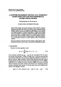
This idea is best illustrated through a simple plot; see Figure 1. These plots depict two different possible relationships between the conditional mean of Y , A and a particular X j , when averaged over all other X i , i  j . Figure 1(a), shows a variable, X1 , which interacts with the action, A , but does not qualitatively interact with the action. Figure 1(b), shows a variable, X 2 , which qualitatively interacts with the action. In both of the plots, the overall optimal action is A = 1 . But in Figure 1(b) there is an apparent reversal of the treatment effect for X 2 values smaller than 0.3 which results in A = 0 being the optimal optimal treatment action for this subset of patients.

Figure 1: Plots demonstrating qualitative and non-qualitative interactions Qualitative treatment-covariate interactions can have a significant influence on the treatment effect while only contributing minimally to the total predictive power of the model. This is the main reason why models based solely on predictive variable selection methods may not work so well when treatment comparison analysis is the application. Proper selection of variables in treatment comparison analysis requires methods which pay special attention to treatment-covariate interactions. Only a small number of methods have been suggested for doing variable selection in this setting (Ernst et al. 2005, Loth et al. 2006, Su et al. 2009, Gunter et al. 2011, Imai and Strauss 2011). A few of these proposed methods are just direct application of predictive variable selection techniques to the particular model (Ernst et al. 2005, Loth et al. 2006). The remaining methods are complicated to use and even more difficult to interpret (Su et al. 2009, Gunter et al. 2011, Imai and Strauss 2011). In this paper we propose a method which is easy to both understand and implement, yet still performs well. While variable selection techniques designed to improve prediction or assess relationships may be directly applied to treatment comparison problems, without adjustment these techniques may neglect certain types of variables that are critical to finding optimal treatments. None-the-less insight can be gained from 366

Pak.j.stat.oper.res. Vol.VII No. 2-Sp 2011 pp363-380

A Simple Method for Variable Selection in Regression with Respect to Treatment Selection

looking at predictive variable selection methods and some of the general ideas utilized by the methods provide a good backbone to build from using new methods more geared toward treatment comparison problems. Predictive variable selection techniques often involve the maximization or minimization of some criterion which weighs the predictive performance of the model as compared to the complexity of the model (Hocking 1976, Tibshirani 1996, Fan and Li 2001) This optimization of criterion can be done either internally or externally from the model fitting process (Guyon and Elisseeff 2003)) . While internal optimization is more efficient, it offers less flexibility in the choice of the criterion that can be used. One category of predictive variable selection methods that offers a great deal of flexibility in its implementation is called Stepwise Regression (Morrison 1967, Pedhazur 1973, Hocking 1976, Lindman and Meranda 1980, Neter et al. 1985, Stevens 1986, Darlington 1990) . Initially proposed by Efroymson (1960), stepwise procedures progressively add or eliminate variables from the predictive model one at a time based on which variable addition or elimination optimizes an external criterion. While the most commonly used stepwise procedure utilizes linear regression for the predictor and p-values or the F-statistic for the optimization criterion (on variables to add or take out), the basic idea defining the procedure can be used much more generally. In particular, any type of predictive model could be used to estimate the response variable and a wide variety of complimentary criteria could be used in the external optimization. Many times we may be interested in regression models where the outcome or response variable is a non-negative integer. The methods that have been previously suggested for doing variable selection in treatment comparison analyses can only be used with a specific type of outcome variable, such as either continuous outcomes (Su et al. 2009, Gunter et al. 2011) or binary outcomes (Imai and Strauss 2011). These methods have not been designed to handle a variety of different outcome variables that we might be interested in using for medical applications where treatment-interaction remains important in the selection of variables. However the simple method we propose is easily applied to a large number of different outcome variables. We apply the simple method successfully in this paper to both logistic regression and Poisson regression, in addition to linear regression. We now provide some background on the types of count models where our proposed method can be used. Many variables in our analysis are categorical, such as educational level, race, hearing loss, etc. Other variables such as age are integers. The common feature of variables such as age is that they take on a finite number of non-negative integer, or count values. Thus when these variables play the role of outcome variables we need a regression model based on a probability distribution that takes into account of the discrete nature of count data. One such model is the Poisson regression model (PRM). Alternatives to PRM are the binomial regression model and the negative binomial regression model, which are based on the binomial and negative binomial probability mass functions respectively. Pak.j.stat.oper.res. Vol.VII No. 2-Sp 2011 pp363-380

367

Lacey Gunter, Michael Chernick, Jiajing Sun

Unlike the Poisson distribution which is equi-dispersed, (i.e. the mean and the variance of a Poisson-distributed random variable are equal) the binomial regression model and the negative binomial regression model can accommodate either under-dispersion or over-dispersion. However, PRM is more commonly used due to its simplicity. As we can see, if a discrete random variable Y has Poisson distribution, then its probability mass function is given by f Y = y  =

exp     y

, y  0,1, 2,... y! By the properties of Poisson distribution, we know EY  =  and VarY  =  . The PRM takes the form that Yi = E Yi    i = i   i ,

where Yi  are a series of independently distributed Poisson random variables with means i and  i  are the stochastic or error terms. In our case the i s are the responses we would like to model. For example say previously we used multiple linear regression to estimate E[Y | X = x; A = a ] , we have Eˆ Y | X = x, A = a  = ˆ 0  x ˆ1  a ˆ2  xa ˆ3 ,

(3)

where A is the treatment variable. In the PRM case, Equation (3) becomes (4) below







Eˆ Y | X = x, A = a  =  ( x, a) = exp ˆ0  xˆ1  aˆ2  xaˆ3 .



(4)

Here exp ˆ0  xˆ1  a ˆ2  xa ˆ3 provides an estimate of the mean value of Y , and since the mean and variance are the same, it also provides an estimate for the variance when the PRM is appropriate. We also note that the model described by Equation 4 is a generalized linear model with link function being the natural logarithm (Nelder and Wedderburn 1972) . The link is the natural logarithm function because it is the inverse of the exponential function which is the necessary transformation to the outcome variable to make it a linear function of the parameters. Again, because many of our variables are nominal rather than numerical, it would be more suitable to use one of the qualitative response regression models. One of the simplest qualitative response regression models is the logit model, which is useful when describing the relationship between the independent variables and a binary response variable. To be more specific when our dependent variable Y is categorical, with Y = 0 denoting being in the 1st category, and Y = 1 being in the 2nd category, we can assume the outcome variable Y is a Bernoulli random variable with the probability of being in the second category, or the probability of `success' being p . Given a set of explanatory variables X , that might inform us about p , we can then model p( x, a) = E Y | X = x, A = a 

368

Pak.j.stat.oper.res. Vol.VII No. 2-Sp 2011 pp363-380

A Simple Method for Variable Selection in Regression with Respect to Treatment Selection

The log of the odds ratio, or the logit, of the probability p ( x , a ) is modeled as a linear function of x and a  p ( x, a )  ˆ ˆ ˆ ˆ LOGIT  p ( x, a )  = ln  (5)  =  0  x 1  a  2  xa  3 . 1  p ( x , a )   The model (5) can also be expressed as 1 p ( x, a ) = . 1  exp   ˆ0  xˆ1  a ˆ2  xa ˆ3    Thus model (5) is then a generalized linear model with a logit link function (Nelder and Wedderburn 1972) .





In the next section, we propose a method which utilizes the basic idea of stepwise procedures, but is geared more toward finding variable subsets which are most useful to the treatment comparison setting. We leave the choice of predictive model up to the user, but suggest an optimization criterion based on the Value function defined in Equation 1. 3. Methods We propose a stepwise variable selection procedure that uses a function of the estimated Value of the optimal policy for the fitted model as a criterion to compare different models. Given an estimated model for the response Y conditional on X and A , an easy way to obtain this estimated Value of the optimal policy is to just optimize the fitted model with respect to the treatment,

Vˆ * = max Eˆ [Y | X = x, A = a].

(6)

a

We refer to this estimator as Vˆ* in our proposed algorithm. Outline of Stepwise variable selection for optimizing treatment: 1. 2. 3. 4. 5. 6.

Fit a model on the treatment action(s) only Estimate the Value of the overall optimal treatment, Vˆ0* by optimizing the treatment only model over the treatment action(s) Define the initial variable set C to contain all known important predictive variables and the treatment variable(s) Estimate the predictive model using all the variables in C Estimate the Value of the optimal policy using the estimated predictive model for C , VˆC* by optimizing the fitted model over the treatment actions Calculate the Adjusted Value of the model for C as AV = (Vˆ *  Vˆ * )/ | C | , C

C

0

7.

where | C | is the rank of the model matrix for model C . At each step perform either a forward selection or backward elimination as follows

(a)

Forward Selection:

Pak.j.stat.oper.res. Vol.VII No. 2-Sp 2011 pp363-380

369

Lacey Gunter, Michael Chernick, Jiajing Sun

Set C = the set of all variables currently in the model and the treatment variable(s) ii. Set E = the set of all eligible predictive variables and all eligible treatment-covariate interactions not currently in the model iii. For each variable e in E i.

A. Estimate the predictive model using all the variables in C plus the variable e using the first data subset B. Estimate the Value of the optimal policy, Vˆe* by optimizing the estimated predictive model over the treatment action(s) C. Calculate the Adjusted Value, AV = (Vˆ *  Vˆ * )/ | C  e | e

e

0

iv. Define e * to be the variable which results in the largest AVe (b)

Backward Elimination Set C = the set of all variables currently in the model and the treatment variable(s) ii. For each variable c in C i.

A. Estimate the predictive model using all the variables in C except the variable c using the first data subset B. Estimate the Value of the optimal policy, Vˆ * by optimizing the c

estimated predictive model over the treatment action(s) C. Calculate the Adjusted Value, AV c = (Vˆ*c  Vˆ0* )/ | C  c | iii. Define c* to be the variable which results in the largest AVc (c)

If AVC < 0 , AV * < 0 and AV * < 0 , exit stepwise method e c

(d)

If AV * > AV C and AV * > AV * , add e * to C and set AV C = AV * e e c e

(e)

If

AV

 c*

> AV C

AV C = AV

8.

and

AV

 c*

> AV

e*

and remove c* from C and set

 c*

If no forward selection or backward elimination can be performed, exit the stepwise method.

The estimated optimal decision rules will only involve the treatment variable(s) and any treatment-covariate interactions present in the model. Thus, the type of variable more likely to lead to an increase in Vˆ * and get added to the model is a treatment-covariate interaction. Predictive variables will only enter the model if they produce a meaningful change in the estimate of the direct effect of treatment or the estimate of the effect of one or more treatment-covariate interactions. For 370

Pak.j.stat.oper.res. Vol.VII No. 2-Sp 2011 pp363-380

A Simple Method for Variable Selection in Regression with Respect to Treatment Selection

this reason we initiate the stepwise method with all known important predictive variables already included in the model. This will give the important predictors a better chance of being included in the final model and will help to ensure better estimates of the effects of treatment throughout. It should be noted that when adding or eliminating any variable from the model it is preferable to maintain a hierarchical ordering (Wu and Hamada 2000). Thus the direct effect of a variable X j should be included in the model anytime the treatment covariate interaction X j A is included in the model, regardless of whether the direct effect has been selected for entry in the model. This will help to avoid including interactions which may only appear important because the direct effect of the covariate is important but omitted from the model. Likewise, it is a good idea to simultaneously add or eliminate variables that come in groups, such as the dummy variables used to code categorical variables with more than two levels. The adjusted Value criterion, AV , used in the algorithm is simply a modification of the Adjusted Gain in Value (AGV) criterion suggested in Gunter et al. (2011) to allow for comparison of non nested subsets. Given a group of nested subsets of variables 1 to K the AGV criterion for the subset of k variables is defined as Vˆk*  Vˆ0*  m  AGVk = *  , Vˆm  Vˆ0*  k  where m = arg max Vˆ * and Vˆ * is the estimated Value of the decision rule k

k

0

ˆ 0* = arg max a Eˆ Y | A = a  . This criterion attempts to trade off between the complexity of a model and its observed Value. It selects the subset of variables that results in the maximum proportionate increase in Value per variable. When doing the above suggested stepwise algorithm, the subsets we are comparing are not nested, so there is not a clear best way to select the model m = arg max k Vˆk* . However, if we assume that there exists a model m* which maximizes Vˆs* among all possible subsets 1,..., S of the full variable set, then this

would be a reasonable choice for m . Then using m* for all subset comparisons our AGV for a subset k would be Vˆk*  Vˆ0*  m*  Vˆk*  Vˆ0*  m*   = AGVk = * . k  Vˆ **  Vˆ0*  Vˆ *  Vˆ0*  k  m  m  But the quantity  m*     Vˆ *  Vˆ *  0   m* is constant for all subsets, thus we can just simplify to Vˆk*  Vˆ0* AVk = k Pak.j.stat.oper.res. Vol.VII No. 2-Sp 2011 pp363-380

371

Lacey Gunter, Michael Chernick, Jiajing Sun

There are several publications which caution about using stepwise procedures for variable selection (Harrell 2001, Miller 2002, Mundry and Nunn 2009). We understand their concerns but would like to address several of the criticisms against stepwise procedures with respect to our proposed method. Most of the arguments against stepwise procedures are directed at versions which use either the p-value of the individual coefficient estimates or the F-statistic for the overall model to determine which variables enter or exit the model. Due to the nature of multiple testing, this type of stepwise procedure suffers from many problems such as inflated coefficient estimates, underestimation of the standard errors of the parameters, overly small p-values, and overly narrow confidence intervals (Harrell 2001, Miller 2002, Mundry and Nunn 2009). Using p-values or the F-statistic to determine stepwise inclusion or exclusion in the model does have drawbacks and we are not recommending it. Our proposed method does not utilize p-values or the F-statistic. Another suggested problem with stepwise procedures is that they do not utilize expert knowledge. Clearly if expert knowledge is available we believe it should be taken into account. We try to incorporate any available expert knowledge concerning good predictors into our proposed method by including them in the initial model. But as was stated earlier, it is very common for experts to which variables are good predictors, but not very common for them to know which variables are good prescriptive variables (possibly because of the lack of familiarity of the concept of prescriptive variables). Our approach can be useful when expert knowledge is lacking. Another problem often cited about stepwise procedures is that not all subsets are tried so there is no guarantee that the optimal subset will be found. This is true of all stepwise procedures, no matter the predictive method or optimization criterion that is used. While this can be a drawback when using a stepwise procedure, there are a couple of reasons why it may still be a better choice than looking at every possible subset, namely computational cost and variability (Hastie et al. 2009) . Clearly as the number of candidate variables increases, it becomes computationally infeasible to compare all possible models. One also pays for the cost of increased variance of the model predictions when checking all possible subsets. Aside from these two issues, the performance between stepwise procedures and checking all possible subsets is often quite similar (Hocking 1976, Hastie et al. 2009). We would also like the reader to note a few other important issues when considering this method. First off, the method is exclusively designed for variable 372

Pak.j.stat.oper.res. Vol.VII No. 2-Sp 2011 pp363-380

A Simple Method for Variable Selection in Regression with Respect to Treatment Selection

selection. The final model estimation procedure should be conducted once important variables have been selected for the model. It is also important to explicitly state that our goal is not to find the optimal predictive model. Thus we not as concerned if good predictors have been excluded from the model, just as long as we are finding the important prescriptive variables and we have precise enough predictor variables to decipher their effects. Excluded predictors that are deemed important may be added to the model during model estimation following variable selection if the user desires. The proposed variable selection procedure can be applied to any modeling technique where a treatment-covariate interaction could be important (e.g. logistic regression, nonlinear regression, Cox proportional hazard regression). For our simulation analysis in the following section we test the method using linear regression, logistic regression and Poisson regression. We also demonstrate the use of the method using data from the Advanced Cognitive Training for Independent and Vital Elderly (ACTIVE) study, a clinical trial conducted to compare alternative cognitive interventions. 4. Simulation Analysis We tested the performance of the new technique in simulations. We used realistically designed simulation data and where applicable, we compared the results to the method proposed in Gunter et al. (2011) referred to as Method S. To generate realistic simulation data, we first randomly selected n = 1401 observation vectors from the baseline observation matrix, X , of the ACTIVE trial data. Information on the data is detailed in Section 5 of the paper. We then generated new treatments, A , by randomly assigning one of two treatments to each row of X . To create the response variable Y we applied 3 different types of outcomes with 4 different generative models for each outcome. The three different types of outcomes we selected are continuous, binary and counts. For the continuous outcomes we randomly selected from 14 outcome variables collected in the ACTIVE trial data. We then added a treatment effect or treatment-covariate interaction to the outcome variable based on the generative model we were using and the new treatments A . We used linear regression to estimate the model. For the binary outcomes, we dichotomize the newly created continuous outcomes from above, using a cutoff of a randomly selected quantile between .3 and .7 . We used logistic regression to estimate the model.

Pak.j.stat.oper.res. Vol.VII No. 2-Sp 2011 pp363-380

373

Lacey Gunter, Michael Chernick, Jiajing Sun

For the counts outcome we randomly selected from 3 outcome variables collected in the ACTIVE trial data that were count variables. We then added a treatment effect or treatment-covariate interaction to the outcome variable based on the generative model we were using and the new treatments A . To ensure the outcomes remained a positive integer, we then rounded the outcomes to the nearest positive integer. We used Poisson regression to estimate the model. The generative models we used are listed below: 1. 2. 3. 4.

No treatment effect and no treatment-covariate interactions; Small treatment effect and no treatment-covariate interactions; One small qualitative treatment-covariate interaction with a binary covariate; One small qualitative treatment-covariate interaction with a continuous covariate.

In generating models 3-4, for each repetition we randomly selected variables from our X matrix to be used in the treatment-covariate interaction. The coefficients for the treatment and qualitative interactions were set such that Cohen's f 2 effect size measure for the treatment effect or the interaction effect was not larger than the suggested definition for `small' of f 2 = .02 (Cohen 1988). For each generated data set, we ran our suggested stepwise method to see which interaction variables were selected by the method. We repeated this 1000 times and recorded the number of spurious interactions selected and whether the true treatment-covariate interaction was selected in models 3 and 4. For the continuous outcomes we also ran Method S and recorded the same information for comparison. The results of our simulations are given in Tables 1 and 2. Table 1 gives the results for the continuous outcome using both our suggested stepwise method and Method S. Table 2 gives the results for the binary and count outcomes for the stepwise method. In both tables the first column lists the generative model used to create the outcome variable. Columns 2 and 3 list the percentage of cases where a spurious treatment-covariate interaction was selected over the 1000 repetitions. Columns 4 and 5 give the average number of spurious interactions selected per repetition. Columns 6 and 7 list the percentage of cases that the true treatment-covariate interaction was selected over the 1000 repetitions. Note that since generative models 1 and 2 have no treatmentcovariate interaction in the generative model, there is no selection percentage for the true treatment-covariate interaction.

374

Pak.j.stat.oper.res. Vol.VII No. 2-Sp 2011 pp363-380

A Simple Method for Variable Selection in Regression with Respect to Treatment Selection

Table 1: Simulation Results for Continuous Outcome. The first column lists the generative model. The next two columns give the percentage of time a spurious interaction was selected by Method S and the Stepwise Method; The next two columns give the average number of spurious interactions selected by both methods over the 1000 repetitions. The last two columns give the selection percentage of the qualitative interaction (when one existed) for each method. Generative Model 1 2 3 4

Spurious Selection Percentage Stepwise Method S 53.3 90.2 21.3 67.3 8.8 6.0 28.4 25.3

Ave # of Spur. Interact. Stepwise Method S 0.852 2.262 0.335 1.870 0.100 0.087 0.377 0.658

Selection Percentage Stepwise Method S 71.9 97.5 48.0 83.8

Looking over Table 1 we see that Method S is better at finding the true treatmentcovariate interaction. As would be expected we lose out a little on performance at the cost of simplicity and generalizability. However, the performance of the stepwise method is not bad and in most of the settings it ended up selecting less spurious interactions than Method S. In Table 2, we see that the performance of the stepwise method is similar and sometimes better when applied to binary and count outcome variables. This demonstrates that the method can be successfully applied to a variety of different outcomes and models. Table 2: Simulation Results for Binary and Count Outcomes. The first column lists the generative model. The next two columns give the percentage of time a spurious interaction was selected by the Stepwise Method for both the binary and count outcome models; The next two columns give the average number of spurious interactions selected for both outcomes over the 1000 repetitions. The last two columns give the selection percentage of the qualitative interaction (when one existed) for each outcome. Generative Model 1 2 3 4

Spurious Selection Percentage Binary Count 86.8 58.7 40.9 6.0 19.1 5.5 31.9 32.4

Ave # of Spur. Interact. Binary Count 1.375 0.967 0.716 0.102 0.279 0.044 0.454 0.454

Selection Percentage Binary Count 79.4 85.9 71.4 46.8

5 Data Example We illustrate the application of the new method on data from a clinical trial. The Advanced Cognitive Training for Independent and Vital Elderly (ACTIVE) study was a randomized controlled trial to test the effects of cognitive interventions on Pak.j.stat.oper.res. Vol.VII No. 2-Sp 2011 pp363-380

375

Lacey Gunter, Michael Chernick, Jiajing Sun

the daily life functions of the elderly (Tennstedt et al. 1999) . The study randomized 2802 people aged 65 or older to one of four treatment groups. The four treatment groups consisted of a control group and three different cognitive interventions. The three cognitive interventions each consist of ten training sessions. One intervention is intended to improve verbal episodic memory, a second is designed to aid inductive reasoning and the third is to help with speed of processing. The study collected several different outcomes to measure daily functioning and cognitive abilities. For more detailed study design and analyses see (Jobe et al. 2001, Ball et al. 2002). We apply the method to two different outcome variables from the data. For both outcomes, we considered 49 baseline variables containing both categorical and quantitative information about the subject's background and current cognitive and health status. All of the variables were considered for both potential predictors and treatment-covariate interactions. For both outcome variables, we used the subset of patients who were randomized to either the verbal episodic memory intervention or the control group. This subset consisted of a total on n = 1401 patients, with 703 assigned to the memory intervention and 698 assigned to the control group. The first outcome variable that we used was the Hopkins Verbal Learning Test (HVLT) total score post treatment. The test was also administered to the patients at baseline. This outcome was a proximal outcome for the verbal episodic memory intervention. We used a linear regression model to fit the data and our initial set of predictors consisted of age, gender, visual acuity, an indicator for hearing loss, a count of the number of medications the patient was taking, the patients Mini Mental Status Exam total score and the baseline HVLT total score. We tried both the stepwise method and Method S on the data. Neither of the methods selected a treatment-covariate interaction, instead opting for the overall optimal treatment being the memory intervention. The second outcome variable that we used was a composite outcome measuring the complex reaction time of the patient post treatment. The patient's complex reaction time was also measured at baseline. Since small reaction times are considered better we used the inverse of the reaction time as our outcome to optimize with respect to treatment. We again used a linear regression model to fit the data and our initial set of predictors consisted of age, gender, visual acuity, an indicator for hearing loss, a count of the number of medications the patient was taking, the patient's Mini Mental Status Exam total score and the baseline complex reaction time. We applied both the stepwise method and Method S on the data. Both of the methods selected a single treatment-covariate interaction with the covariate being the baseline complex reaction time. The interaction appeared to suggest the overall optimal treatment was the memory intervention, but smaller baseline complex reaction times showed the treatment to be no more effective than no 376

Pak.j.stat.oper.res. Vol.VII No. 2-Sp 2011 pp363-380

A Simple Method for Variable Selection in Regression with Respect to Treatment Selection

treatment at all. This may be the case because there is a floor on the complex reaction times for the patient population so if the patient is near that floor at baseline the reaction times have little to no ability to improve regardless of the treatment. 6. Discussion In this article, we proposed a simple method for doing variable selection when the goal is to compare and optimize treatments. The method is a variant of stepwise regression that can be applied quite generally to a variety of predictive treatment models. While the method does result in a small loss in performance over more complex methods, it does surprisingly well for its level of simplicity and generalizability. As might be expected the suggested method sometimes includes interaction variables which are spurious. This was seen in the simulation results. When applying this method to a real data set for analysis, it might be advisable to incorporate some form of cross-validation or bootstrap validation to the algorithm if it is important to minimize or control the number or percentage of false discoveries (Gong 1986, Chernick 2007). The proposed method is an attempt to create a variable selection technique that can be easily applied and used with a variety of different types of response variables such as binary and count. These are the big advantages of this new stepwise method: We have many ideas for future research. One avenue we would like to explore is to modify the way we generate the models for binary and count data and see how it affects the results. An alternative way to build the generative model would be to pick one that fits perfectly with the linear regression model, and then generate the count and binary variables according to the link functions. For the logit model, we could generate the probabilities and then generate the response variables according to that probability measure. Also alternative ways of modeling count data could be explored, such as integervalued autoregressive process (INAR). An INAR model is similar to an AR model in correlation structure under binomial thinning (Du and Li 1991) , so instead of assuming that the treatment effect is multiplicative, we could assume the treatment effect to be a binomial thinning operator. To be more specific, instead X of AX we could use A  X , where A  X = i =1Bit where B1t , B 2t ,  , B X t are t 1

i.i.d. Bernoulli random variables with P (Bit = 1) = 1  P (Bit = 0) = A , i.e. A  X has, conditional on X , a binomial distribution with parameters A and X . If we use this data generating process, we could ensure that the data are made of integers, and the correlation structures are the same as AX , because the binomial distribution is discrete by nature and EA  X  = AX . Another avenue we would like to explore is trying the method out on Cox proportional hazards model and nonlinear regression models and other types of time related models such as harmonic regression.

Pak.j.stat.oper.res. Vol.VII No. 2-Sp 2011 pp363-380

377

Lacey Gunter, Michael Chernick, Jiajing Sun

References 1.

Ball, K., Berch, D.B., Helmers, KF, Jobe, J.B., Leveck, M.D., Marsiske, M., Morris, J.N., Rebok, G.W., Smith, D.M., Tennstedt, S.L., Unverzagt, F.W.,& Willis, S.L. (2002). “Effects of cognitive training interventions with older adults: a randomized controlled trial." Journal of the American Medical Association, 288, pp. 2271-2281.

2.

Chernick, M.R. (2007). Bootstrap Methods: A Guide for Practitioners and Researchers, 2nd edn., Wiley, Hoboken.

3.

Cohen J. (1988), Statistical Power Analysis for the Behavioral Sciences, 2nd edn., Lawrence Earlbaum Associates, Hillsdale, NJ.

4.

Darlington, R.B. (1990). Regression and linear models, McGraw-Hill, New York.

5.

Draper, N.R. & Smith H. (1981). Applied Regression Analysis, 3rd edn., Wiley, New York.

6.

Du, J. & Li Y. (1991). The integer-valued autoregressive (INAR(p)) model, Journal of Time Series Analysis, 12(2), pp. 129-142.

7.

Efroymson, MA (1960). Multiple regression analysis. In Ralston, A. and Wilf, HS, editors, Mathematical Methods for Digital Computers. Wiley.

8.

Ernst, D., Geurts, P. & Wehenkel, L. (2005). Tree-based batch mode reinforcement learning, Journal of Machine Learning Research, vol. 6, pp. 503-556.

9.

Fan, J. & Li, R. (2001). Variable Selection via Nonconcave Penalized Likelihood and Its Oracle Properties, Journal of the American Statistical Association, 96(456), pp. 1348-1360.

10.

Gong, G. 1986, Cross-validation, the jackknife, and the bootstrap: Excess error in forward logistic regression, Journal of the American Statistical Association, vol. 81, no. 393, pp. 108-113.

11.

Gunter, L., Zhu, J. & Murphy, S.A. (2011). Variable selection for qualitative interactions, Statistical Methodology, 8(1), pp. 42-55.

12.

Guyon, I. & Elisseeff, A. (2003). An introduction to variable and feature selection, The Journal of Machine Learning Research 3, pp. 1157-1182.

13.

Harrell, F.E. (2001). Regression modeling strategies: With Applications to Linear Models, Logistic Regression, and Survival Analysis, SpringerVerlag, New York.

14.

Hastie, T., Tibshirani, R. & Friedman, J. (2009). The Elements of Statistical Learning: Data Mining, Inference, and Prediction, 2nd edn., Springer-Verlag.

15.

Hocking, R.R. (1996). Methods and Applications of Linear Models: Regression and the Analysis of Variance, 2nd Edition, Wiley, New York.

16.

Hocking, R.R. (1976). A Biometrics Invited Paper. The Analysis and Selection of Variables in Linear Regression, Biometrics, 32(1), pp. 1-49.

378

Pak.j.stat.oper.res. Vol.VII No. 2-Sp 2011 pp363-380

A Simple Method for Variable Selection in Regression with Respect to Treatment Selection

17.

Horvitz, D.G. & Thompson, D.J. (1952). A Generalization of Sampling Without Replacement From a Finite Universe, Journal of the American Statistical Association 47(260), pp. 663-685.

18.

Imai, K. & Strauss, A. (2011). Estimation of Heterogeneous Treatment Effects from Randomized Experiments, with Application to the Optimal Planning of the Get-Out-the-Vote Campaign, Political Analysis, 19(1), pp. 1-19.

19.

Jobe, J.B., Smith, D.M., Ball, K., Tennstedt, S.L., Marsiske, M., Willis, S.L., Rebok, G.W., Morris, J.N., Helmers, K.F., Leveck, M.D. & Kleinman, K. (2001). ACTIVE: a cognitive intervention trial to promote independence in older adults. Controlled Clinical Trials, 22, pp. 453-479.

20.

Lindeman, R.H., Merenda, P.F. & Gold, R. (1980). Introduction to bivariate and multivariate analysis, Scott, Foresman, & Co., New York.

21.

Loth, M., Davy, M. & Preux, P. (2006). Sparse temporal difference learning using lasso, in: IEEE International Symposium on Approximate Dynamic Programming and Reinforcement, Springer, Hawaii, USA.

22.

Miller, A.J. (2002). Subset selection in regression, Chapman & Hall, London.

23.

Morrison, D. (1967). Multivariate statistical methods, McGraw-Hill, New York.

24.

Mundry, R. & Nunn, C. 2009, Stepwise Model Fitting and Statistical Inference: Turning Noise into Signal Pollution., The American Naturalist, 173(1), pp. 119-123.

25.

Neter, J., Wasserman, W. & Kutner, M.H. (1985). Applied linear statistical models: Regression, analysis of variance, and experimental designs, 2nd edn, Richard D. Irwin, Inc, Homewood, IL.

26.

Nelder, J.A. & Wedderburn, R.W.M. (1972). Generalized Linear Models. Journal of the Royal Statistical Society, Series A, 135, pp. 370-384.

27.

Pedhazur, E.J. (1973). Multiple regression in behavioral research, Holt, Rinehart, & Winston, New York.

28.

Peto, R. Statistical aspects of cancer trials. In K. Halnan, (1982). Treatment of Cancer, pages 867--871. Chapman and Hall, London, UK

29.

Rubinstein, R.Y. (1981). Simulation and the Monte Carlo Method, Wiley, New York.

30.

Stevens, J. (1986). Applied multivariate statistics for the social sciences, Erlbaum, Hillsdale, NJ.

31.

Su, X., Tsai, C., Wang, H., Nickerson, D.M. & Li, B. (2009). Subgroup Analysis via Recursive Partitioning, Journal of Machine Learning Research, 10, pp. 141-158.

32.

Sutton, R.S. & Barto, A.G. (1998). Reinforcement Learning: An Introduction, MIT Press, Cambridge, MA.

Pak.j.stat.oper.res. Vol.VII No. 2-Sp 2011 pp363-380

379

Lacey Gunter, Michael Chernick, Jiajing Sun

33.

Tennstedt, S., Morris, J., Unverzagt, F., Rebok, G., Willis, S., Ball, K., & Marsiske, M. 1999-2001, ACTIVE (Advanced Cognitive Training for Independent and Vital Elderly), [United States] [Computer file]. ICPSR04248-v3. Ann Arbor, MI: Inter-university Consortium for Political and Social Research [distributor], 2010-06-30. doi:10.3886/ICPSR04248.

34.

Tibshirani, R. (1996). Regression Shrinkage and Selection via the Lasso, Journal of the Royal Statistical Society. Series B (Methodological), 58(1), pp. 267-288.

35.

Wu, C.F. & Hamada, M. (2000). Experiments: Planning, Analysis, and Parameter Design Optimization, Wiley, New York.

36.

Yan, X. & Su, X. (2005). Testing for qualitative interaction. In S. C. Chow, editor, Encyclopedia of Biopharmaceutical Statistics. Informa Health Care

37.

Younger, M.S. (1985). A first course in linear regression, 2nd ed, Duxbury Press, Boston.

380

Pak.j.stat.oper.res. Vol.VII No. 2-Sp 2011 pp363-380