JOURNAL OF CHEMICAL PHYSICS
VOLUME 116, NUMBER 7
15 FEBRUARY 2002
A simple molecular thermodynamic theory of hydrophobic hydration Henry S. Ashbaugh Department of Chemical Engineering, Princeton University, Princeton, New Jersey 08544 and Los Alamos National Labs, Group T12, Mail Stop B268, Los Alamos, New Mexico 87545
Thomas M. Truskett Department of Pharmaceutical Chemistry, University of California-San Francisco, San Francisco, California 94118 and Department of Chemical Engineering, The University of Texas at Austin, Austin, Texas 78712
Pablo G. Debenedettia) Department of Chemical Engineering, Princeton University, Princeton, New Jersey 08544
共Received 25 July 2001; accepted 27 November 2001兲 A recently developed microscopic model for associating fluids that accurately captures the thermodynamics of liquid water 关Truskett et al., J. Chem. Phys. 111, 2647 共1999兲兴 is extended to aqueous solutions with nonpolar species. The underlying association model incorporates the highly directional and open nature of water’s hydrogen-bond network, and, as a result, captures a number of the distinguishing properties of liquid water, such as the density anomaly. The model for aqueous mixtures developed herein predicts many of the thermodynamic signatures of hydrophobic hydration without resorting to empirical temperature-dependent parameters. The predicted solubility of nonpolar species is slight over a wide range of temperatures, and exhibits a minimum as a function of temperature, in accord with experiment. Hydration is opposed by a dominant entropy and favored by the enthalpy at low temperatures. At elevated temperatures these roles are reversed. Furthermore, the hydration entropies for hydrophobes of varying size converge over a very narrow temperature range. Comparison with experimental and simulation data for nonpolar solutes in water shows that the theory tends to exaggerate the solute’s transfer heat capacity at low temperature, and hence solubility minima and entropy convergence are predicted to occur at lower temperatures than observed. Our results support the emerging view that hydrophobic effects can be attributed in large part to the equation of state for pure water. © 2002 American Institute of Physics. 关DOI: 10.1063/1.1436479兴
larly undergo hot and cold denaturation,4,5 while ionic and nonionic surfactants display a minimum in their critical micelle concentrations with respect to temperature,6,7 suggesting a common underlying mechanism. Careful analysis of the experimental entropies of hydrocarbon hydration as a function of temperature reveals that these curves intersect at an entropy close to zero at approximately 385 K.8 –14 The coincidence of this entropy convergence temperature with comparable behavior in protein unfolding has been taken as a thermodynamic foundation for the hydrophobic core model for protein folding. The ability to predict and reproduce the features described above may be considered essential for models of hydrophobic effects involving simple solutes. Traditionally, it has been argued that hydrophobic effects result from the orientational constraints in the hydration shell of a nonpolar solute as a result of water’s attempt to maintain the integrity of the hydrogen-bonding network by forming clatharatelike structures or microscopic ‘‘icebergs.’’ 15 While providing a convenient language for discussing hydrophobic hydration, this interpretation does not resolve the relative magnitudes of the opposing enthalpic and entropic contributions, and belies the richness of their temperature dependencies. Experimental probes of vicinal water structure are scarce, in large part because of the low solute concentrations involved.16 –21 The structures that have been measured sug-
I. INTRODUCTION
The meager solubility of nonpolar hydrophobic molecules in water is upheld as the primary thermodynamic driving force for a number of important aqueous solution phenomena, including the environmental fate of pollutants, surfactant micellization, biological membrane formation, and the folding of globular proteins.1–3 Beyond the adage ‘‘oil and water do not mix,’’ molecular-scale hydrophobic effects are associated with a number of key thermodynamic fingerprints.1 Dissolution heats determined from calorimetric studies indicate that unfavorable entropies of transferring nonpolar gases into water dominate hydration free energies at room temperature, and are only partly compensated by favorable dissolution enthalpies. These entropies and enthalpies are strongly temperature dependent, as indicated by large positive transfer heat capacities. At elevated temperatures, the roles of entropy and enthalpy are reversed, with unfavorable enthalpies dominating hydration free energies, partly compensated by favorable entropies. The resulting solubilities of nonpolar gases are nonmonotonic, passing through a minimum between 310 and 350 K. Proteins simia兲
Author to whom correspondence should be addressed. Electronic mail:
[email protected]
0021-9606/2002/116(7)/2907/15/$19.00
2907
© 2002 American Institute of Physics
Downloaded 13 Feb 2002 to 128.112.35.162. Redistribution subject to AIP license or copyright, see http://ojps.aip.org/jcpo/jcpcr.jsp
2908
J. Chem. Phys., Vol. 116, No. 7, 15 February 2002
gest that while water adopts orientational preferences in the hydration shell of nonpolar moieties, the solute induced structure in water is somewhat more disordered than that in ice or clatharate hydrates.16 –20 To date, molecular level investigations of hydrophobic hydration have been mostly theoretical and computational.22– 42 Extensions of scaled particle theory to hydrophobic hydration, for example, have provided a molecular rationale for the application of surface area models down to microscopic length scales.43– 48 The correlation between macroscopic and microscopic surface tensions, however, is contentious due to differences in their temperature dependencies.1 Water structure and orientational preferences in the vicinity of hydrophobic species has been connected to the characteristic entropies of hydrophobic hydration through the application of a statistical mechanical correlation function expansion for the entropy.22,49–51 More recently, information theory 共IT兲, with roots in Pratt–Chandler52 and Gaussian field theory,53 has provided a quantitative link between the microscopic density fluctuations determined from water oxygen pair correlations and the hydration free energies of hard solutes. More importantly IT implicates the density and isothermal compressibility of water—macroscopic equation of state properties—as dominant factors in hydrophobic hydration. In addition to capturing temperature26 and pressure30 effects associated with hydrophobic hydration and interactions, IT provides an explanation of the slightly greater solubility of nonpolar species in heavy water compared to light water as a result of differences in the isothermal compressibilities of these two solvents.31 Although IT is a useful and original approach for the analysis and interpretation of solvation phenomena, it is not a predictive theory for the solubility of nonpolar solutes. Equations of state 共EOS兲 can accurately describe the solubility of water in organic liquids, yet they fail to capture the solubility of nonpolar solutes in water 共e.g., hydrocarbons兲 or the nonmonotonic temperature dependence of the solubility.54 –56 In light of IT considerations, it appears reasonable that an appropriate starting place for developing an accurate EOS model for the dissolution of nonpolar solutes in water would be an accurate EOS for water itself. Typically, engineering EOS for water must rely on ad hoc temperature dependent parameterizations to accurately model the liquid state anomalies 共e.g., negative thermal expansion兲, limiting potential physical insights as well as predictive capabilities. Recently, however, Truskett et al. developed a new partition function and EOS for water.57 A key feature of their theory is the incorporation of a positive correlation between entropy and density in the vicinity of a hydrogenbonded molecule. This schematic and simplified incorporation of the cooperativity of hydrogen-bond formation captures many of the characteristic anomalies of liquid water including the density maximum at 4 °C and isothermal compressibility minimum. In this work, we generalize this model to mixtures with nonhydrogen-bonding hydrophobic solutes. The analytical partition function for mixtures captures the salient features of hydrophobic hydration summarized above, and provides insights into their origin. The present molecular theory captures the thermodynamic signatures of hy-
Ashbaugh, Truskett, and Debenedetti
drophobic hydration without resorting to empirical temperature dependencies58,59 or treatments of hydrogenbonding,60,61 demonstrating that a realistic EOS for water provides a sound and natural foundation for describing aqueous mixtures with nonpolar molecules. Moreover, the present theory is not limited to infinite dilution62 and can potentially impact the prediction of the phase behavior of oil–water mixtures at finite concentrations. II. THEORETICAL DEVELOPMENT A. Derivation of the mixture partition function
In a preceding study, a statistical mechanical model of associating fluids was proposed.57 The resulting EOS captures many of water’s thermodynamic anomalies 共e.g., negative thermal expansion, compressibility minima, increase in the isobaric heat capacity upon cooling, liquid–liquid phase transition兲 with remarkable success. The theoretical premise of this model is to treat the formation of a hydrogen-bond in detail, and to incorporate, in an approximate fashion, the cooperative consequences due to the directionality of the bonds. In particular, a pair of water molecules participating in a hydrogen-bond must posses mutually favorable orientations and a sparse low-density environment in the vicinity of the bond. The basic physical attributes of the hydrogen-bond are summarized as follows 共see also Fig. 1兲: 共1兲 One of the two interacting water molecules, denoted as the central water molecule, must be surrounded by an exclusion shell of radius r wi devoid of any other waters. In this way the theory incorporates, albeit in a schematic fashion, the fact that the tetrahedral arrangement of a fully hydrogen-bonded molecule and its four participating neighbors results in an open, low-density environment, in contrast with the 12-fold coordination of atomic liquids. 共2兲 A hydrogen-bonding pair of water molecules must be separated by a distance, r, that lies within the hydrogen bonding shell, r wi ⬍r⬍r w0 , of the central water molecule. The width of this shell represents the librational degree of freedom of a hydrogen-bond. 共3兲 The bonding pair must have mutually favorable orientations, such that 1 and 2 ⬍ * . 共4兲 The presence of additional water molecules in the hydrogen-bonding shell ‘‘crowds’’ and weakens the existing bond. An energy of ⫺ max is assigned to a solitary bonding pair, with a penalty of pen for each nonbonding molecule in the shell. These hydrogen-bonding criteria in conjunction with the mean-field approximation for dispersion interactions, and the van der Waals 共vdW兲 prescription for excluded volume interactions lead to the following expression for the partition function for water (w), Q 共 N w ,V,T 兲 ⫽ 共 N W !⌳ w w 兲 ⫺1 共 V⫺N w b w 兲 N w 3N
j max
⫻exp共  N w2 a ww /V 兲 (4 ) N w
兿
j⫽1
f 共 j 兲 Nw p共 j 兲. 共1兲
A detailed derivation of this partition function can be found in Ref. 57. In this expression ⌳ w is the thermal wavelength,
Downloaded 13 Feb 2002 to 128.112.35.162. Redistribution subject to AIP license or copyright, see http://ojps.aip.org/jcpo/jcpcr.jsp
J. Chem. Phys., Vol. 116, No. 7, 15 February 2002
Theory of hydrophobic hydration
2909
energy are not independent, and some of the quantities in the ‘‘hydrogen-bond’’ term, such as p( j), contain hard sphere 共excluded volume兲 information exclusively. A detailed discussion of the occupation probabilities is presented below. Returning to Eq. 共1兲 f ( j) arises from the orientational contributions to the hydrogen-bonding partition-function for a central water molecule with j water molecules in its bonding shell 共r wi ⬍r⬍r wo in Fig. 1兲 and is given by j f 共 j 兲 ⫽1⫹ 共 1⫺cos * 兲 2 兵 exp关  共 j 兲兴 ⫺1 其 . 4
共3兲
( j) is the hydrogen-bonding energy between a pair of water molecules when there are ( j⫺1) crowding water molecules in the bonding shell of the central molecule, ⫺ 共 j 兲 ⫽⫺ max⫹ 共 j⫺1 兲 pen .
FIG. 1. Schematic illustration of the microscopic model. 共a兲 In order to form a hydrogen bond, two water molecules must be properly oriented, with their bonding directions pointing towards each other ( 1 , 2 ⬍ * ), regardless of the value of 1 and 2 . 共b兲 Water molecules have a hard core of radius ww , within which the center of no other water molecule can penetrate. In order to form a hydrogen bond, positional constraints must be satisfied in addition to the orientational requirements shown in 共a兲. Specifically, a central water molecule must be surrounded by an exclusion shell of radius r wi , devoid of centers of other water molecules, and a properly oriented second water molecule must be inside its hydrogen bonding shell (r wi ⭐r⭐r wo ). The presence of additional molecules within the hydrogen bonding shell weakens an existing bond. 共c兲 Water–solute interactions. Water molecules 共gray兲 have a hard core radius sw ⫽( ww ⫹ ss)/2, within which the center of no other nonpolar solute 共white兲 can penetrate. In order to form a hydrogen bond, a central water molecule must be surrounded by a solute exclusion shell of radius r si . Solutes whose centers lie in the hydration shell (r si ⭐r ⭐r so ) can affect the strength of a hydrogen bond.
共4兲
The above-described model and its generalization to mixtures capture the distinctive features of the thermodynamics of water and of its mixtures with nonpolar solutes. Nevertheless, drastic simplifications are introduced in the description of hydrogen bonds. Consequently, ours is not a microscopic theory of water structure around nonpolar solutes. Rather, our work suggests that the complex macroscopic behavior commonly referred to as hydrophobic hydration can be adequately described as long as a positive correlation between local entropy, density, and energy is incorporated into a microscopic theory of water. This is what the above fourpoint description of hydrogen bond formation accomplishes, once translated into the language of statistical mechanics. As shown in Appendix A, the partition function for water can be readily generalized to aqueous mixtures with nonpolar species 共s兲 as Q 共 N w ,N s ,V,T 兲 ⫽ 共 N w !N s !⌳ w w ⌳ s s 兲 ⫺1 共 V⫺Nb 兲 N 3N
N w is the number of water molecules, V is the volume, T is the temperature, and  ⫺1 ⫽kT is the product of Boltzmann’s constant and the temperature. a ww and b w are the familiar vdW attractive parameter for water–water pair interactions, and the excluded volume per water molecule of hard core diameter ww , respectively. We require the pressure to diverge at the random close packing density 0.64b w ⫽
3 ww , 6
共2兲
where the spheres occupy 64% of the volume. It should be noted that the use of the simple one-dimensional approximation for the excluded volume is not necessary for the theory. More accurate expressions for the excluded volume, e.g., Carnahan–Starling,63 produce similar predictions. The first three terms in the product on the right-hand side of Eq. 共1兲 comprise the partition function of a vdW fluid. The last two terms then constitute the contribution of aqueous hydrogen-bonding. p( j) is the probability that j water molecules occupy the bonding shell and that the exclusion shell 共 ww ⬍r⬍r wi in Fig. 1兲 is devoid of water molecules. The maximum number of water molecules allowed in the bonding shell is j max . Note that in the original derivation the hydrogen-bonding and hard sphere contributions to the free
3N
⫻exp共  N 2 a/V 兲 j max k max
⫻共 4 兲
Nw
兿兿
j⫽1 k⫽0
f 共 j,k 兲 N w p 共 j,k 兲 .
共5兲
In the limit N s →0 this expression reduces to the partition function for pure water 关Eq. 共1兲兴, while in the limit N w →0 it reduces to the partition function of a vdW fluid. Standard mixing rules are applied to evaluate the mixed vdW a and b parameters, a⫽x w2 a ww ⫹2x w x s a sw ⫹x s2 a ss ,
共6a兲
b⫽x w b w ⫹x s b s ,
共6b兲
where x i ⫽N i /N is the mole fraction of species i, and the cross solute–water vdW interaction parameter is a sw ⫽(a ww a ss ) 1/2. It remains to describe below the effect of the nonpolar species on the hydrogen-bonding contributions to the partition function. Hydrogen-bonding interactions in these mixtures should take into account the fact that while the nonpolar species cannot hydrogen-bond with water, they can potentially stabilize or destabilize bonding between water pairs through perturbations in the bonding energy. By analogy with the model for pure water 共Fig. 1兲, we assume there is an inner shell
Downloaded 13 Feb 2002 to 128.112.35.162. Redistribution subject to AIP license or copyright, see http://ojps.aip.org/jcpo/jcpcr.jsp
2910
J. Chem. Phys., Vol. 116, No. 7, 15 February 2002
Ashbaugh, Truskett, and Debenedetti
surrounding the central water molecule ( sw ⬍r⬍r si ) devoid of solute molecular centers, referred to as the solute exclusion shell, and an outer shell (r si ⬍r⬍r so ) within which the solute can affect hydrogen-bonding, referred to as the solute hydration shell. For j water molecules in the bonding shell and k solute molecules in the solute hydration shell, the central water molecule’s orientational contribution to its hydrogen-bonding partition function 共see Appendix A兲 is given by j f 共 j,k 兲 ⫽1⫹ 共 1⫺cos * 兲 2 兵 exp关  共 j,k 兲兴 ⫺1 其 . 4
where ⫽ w ⫹ s , the total number density, is the sum of the water and solute number densities. In the limits w →0 or s →0 this expression reduces to the vdW EOS or the EOS for pure water given in Ref. 57, respectively. The solute chemical potential is determined by the solute number derivative of the Helmholtz free energy,
s⫽
冉 冊 A Ns
⫽⫺kT T,V,N w
共7兲
p 共 j,k 兲 ⫽p 0 p w 共 j 兲 p s 共 k 兲 .
共9兲
p 0 is the probability that a central water molecule has its exclusion shells ww ⬍r⬍r wi and sw ⬍r⬍r si devoid of water and solute molecules. p w ( j) is the conditional probability that there are j water molecules in the central water’s hydrogen bonding shell (r wi ⬍r⬍r wo ) given that the exclusion shells are devoid of water and nonpolar species. p s (k) is analogous to p w ( j), and denotes the conditional probability of observing k nonpolar molecules in the solute hydration shell (r si ⬍r⬍r so ) given that the exclusion shells are devoid of water and nonpolar species. The detailed mathematical expressions for p 0 , p w ( j), and p s (k) are presented in Appendix B.
The thermodynamic properties of aqueous mixtures can be determined from the partition function 关Eq. 共5兲兴. The first quantity we consider is the EOS, which is given by the volume derivative of the Helmholtz free energy,
冉 冊 冉 冊
⫽kT
⫽
A V
T,N w ,N s
ln Q V
共10a兲
, T,N w ,N s
kT ⫺a 2 ⫹kTN w 1⫺ b j max k max
⫻
兺兺 j⫽1 k⫽0
再冋 册 p 共 j,k 兲 V
冎
ln f 共 j,k 兲 , N w ,N s
j max k max
⫻
兺兺 j⫽1 k⫽0
再冋
p 共 j,k 兲 s
共10b兲
册
kT b s 1⫺ b
冎
ln f 共 j,k 兲 . w
共11b兲 A useful way of expressing the solubility of a gas in water is by the Ostwald solubility 共L兲 defined as66 L⫽
s , sg
共12兲
where the superscript g indicates the gas phase. Assuming that the gas phase behaves ideally, sig ⫽kT ln sg⌳s3, it follows from equating the chemical potential of the solute in the ideal gas and solution phase at the given T and P, sig ⫽ saq , that ⫺ln L⫽  s* ,
共13兲
where s* , the excess solute chemical potential, contains the nonideal contributions to the chemical potential in the aqueous phase, that is to say the second, third, fourth, and fifth terms on the right-hand side of Eq. 共11b兲. The individual terms in the chemical potential expression can be broken down into point creation,43 excluded volume, attractive, and hydrogen-bonding contributions,
* ⫹ s,vol * ⫹ s,att * ⫹ s,hb * . s* ⫽ s,pt
B. Evaluation of thermodynamic properties of aqueous solutions
P⫽⫺
共11a兲 T,V,N w
⫺2 共 w a sw ⫹ s a ss兲 ⫺kT w
共8兲
where np is the nonpolar energetic contribution per solute molecule in the hydration shell.15,64,65 The other important quantity introduced in the mixture partition function is p( j,k), the probability that the central molecule is surrounded by j water molecules and k solute molecules satisfying the positional criteria for hydrogenbond formation. The key simplifying assumption that we make is that this quantity can be expressed as a superposition of independent solvent and solute occupation probabilities,
ln Q Ns
⫽kT ln s ⌳ s3 ⫺kT ln共 1⫺ b 兲 ⫹
The hydrogen-bonding energy in this case is ⫺ 共 j,k 兲 ⫽⫺ max⫹ 共 j⫺1 兲 pen⫹k np ,
冉 冊
共14兲
The infinite dilution limits of these quantities, * ⬁ , s,vol * ⬁ , s,att * ⬁ , s,hb * ⬁ are given in Appendix C. Infinite di s,pt lution quantities are of interest in the present context because * ⬁ is the of the low solubility of nonpolar solutes in water. s,pt reversible work associated with inserting a hard pointlike * ⬁ is the reversible work associated solute in solution,43 s,vol with growing the pointlike solute to its full diameter ss , * ⬁ is the reversible work associated with turning on attrac s,att * ⬁ is the reversible tive solute–water interactions, and s,hb work associated with restructuring water’s hydrogen-bond network upon introducing the solute. We denote the additive contribution arising from orientation-dependent interactions as the hydrogen-bonding term. It should be understood, however, that in the present theory it is impossible to separate completely the hydrogen-bond and HS terms, since the angular integrals are evaluated in the HS ensemble 共see Appendix A兲, and p 共j, k兲 contains exclusively HS terms, i.e., G mn 共Appendix B兲.
Downloaded 13 Feb 2002 to 128.112.35.162. Redistribution subject to AIP license or copyright, see http://ojps.aip.org/jcpo/jcpcr.jsp
J. Chem. Phys., Vol. 116, No. 7, 15 February 2002
Theory of hydrophobic hydration
By differentiating the chemical potential with respect to temperature at constant pressure, the partial molar excess enthalpy and entropy can be derived. The enthalpy is given as ¯h s* ⫽⫺T 2
冉
s* /T T
冊
¯ s,pt ¯ s,vol ¯ s,att ¯ s,hb * ⫹h * ⫹h * ⫹h * . ⫽h P,N w ,N s
共15兲
Note that the pressure is an independent variable in the partial derivative shown in Eq. 共15兲. The present theory was developed in the canonical ensemble, where volume, not pressure, is the independent variable. The calculation of partial derivatives such as Eq. 共15兲 is discussed in Appendix D. The individual contributions to the partial molar enthalpy in the limit of infinite dilution are given in Appendix C. The entropy is given as ¯s s* ⫽⫺
冉 冊 s* T
* ⫹s¯ s,vol * ⫹s¯ s,att * ⫹s¯ s,hb * , ⫽s ¯ s,pt
共16兲
P,N w ,N s
where the individual contributions to the partial molar entropy in the limit of infinite dilution are, once again, given in Appendix C. C. Model parameterization
In the original paper introducing this model for pure water,57 the parameters max , pen , w , and a ww were fixed. The magnitude of the maximum hydrogen bond strength max and the hard core diameter w were set at the physically reasonable values of 23 kJ/mol and 3.11 Å, respectively. The crowding penalty pen was set to 3 kJ/mol per nonbonding molecule in the hydrogen bonding shell. The dispersion interaction a ww was set so as to give the correct critical temperature for water. The remaining parameters, r wi , r wo , and * were used as variables. Two parameter sets were explored by varying * and using r wi and r wo to reproduce the density maximum at 4 °C and 1 g/cm3. It was found that the parameter set that resulted in phase behavior with a second critical point in the deeply supercooled region67–73 共 * ⫽0.175 rad, r wi ⫽1.01 w , r wo ⫽1.04 w 兲 provided the best fit to water’s ( P,V,T) behavior. In this work we adopt this parameter set, although we have adjusted a ww , ww , and r wi to compensate for the simplifications 关Eqs. 共B3兲–共B5兲兴 introduced in the expressions for the bonding shell occupation probabilities, and to improve the fit to the density of liquid water at atmospheric pressure. These parameters are listed in Table I. The fitted density and thermal expansion coefficient of liquid water are shown in Fig. 2. These adjusted parameters still conform to the two-critical-point scenario, however, the gas–liquid critical point has been shifted to ⬃50 K above the experimental value. This is predominantly a result of the increase in the a ww parameter. The present study focuses on temperatures well below the critical temperature and this is not considered further. Nonpolar solutes have been found to stabilize hydrogen bonds.20,64,65,74,75 However, rather than introducing additional parameters associated with the effect of a hydrophobe on hydrogen-bonding, we assume np⫽0 and r si ⫽r so ⫽ sw . We have conducted a preliminary study of the
2911
TABLE I. Model parameters for water and its mixtures.
ww r wi r wo a ww * max pen j max r si r so np k max
3.135 Å 1.008 ww 1.04 ww 0.310 Pa m6/mol2 0.175 rad 23 kJ/mol 3 kJ/mol 8 sw sw 0 8
effect of these terms and find that they have little influence on the predicted solubility trends. Thus, the present study focuses on the effect of the solute size and attractive interactions on the thermodynamics of hydrophobic hydration. A detailed parametric analysis of the effects of hp , ss , r si , and r so on the calculated solubility is underway and will be published separately. III. RESULTS AND DISCUSSION
The temperature dependence of the chemical potential of a ss⫽4 Å spherical solute at infinite dilution at atmospheric pressure is shown in Fig. 3. The top curve is s* ⬁ for a HS solute (a sw ⫽0), while the remaining curves indicate increasing solute-water attractive interactions 共a sw varying from 0 to 0.25 Pa m6 mol⫺2兲. It can be seen that  s* ⬁ passes through a maximum, or equivalently the Ostwald solubility
FIG. 2. Temperature dependence of the density 共a兲 and thermal expansion coefficient 共b兲 of water at atmospheric pressure. The points are experimental data 共Refs. 90, 91兲. The line is the model prediction for pure water, using the parameters of Table I.
Downloaded 13 Feb 2002 to 128.112.35.162. Redistribution subject to AIP license or copyright, see http://ojps.aip.org/jcpo/jcpcr.jsp
2912
J. Chem. Phys., Vol. 116, No. 7, 15 February 2002
FIG. 3. Model prediction for the temperature dependence of the dimensionless excess chemical potential of a hydrophobic solute ( ss⫽4 Å) in water, at atmospheric pressure and infinite dilution (  ⫽1/kT). The top curve corresponds to a hard sphere 共HS兲 solute (a sw ⫽0). Each successive curve corresponds to an increment in the solute–solvent van der Waals attractive parameter, a sw , of 0.05 Pa m6 mol⫺2. The dotted line shows the locus of maxima in the dimensionless chemical potential, with attractive interactions 共i.e., a sw 兲 increasing in the direction of the arrow. Maxima in the dimensionless chemical potential are equivalent to minima in the infinite dilution limit of the Ostwald solubility 关Eq. 共13兲兴.
关Eq. 共13兲兴 at infinite dilution passes through a minimum. For the HS solute the solubility minimum 共268 K兲 occurs close to the density maximum of pure water 共277 K兲. Indeed, these two temperatures would coincide if  s* ⬁ was determined solely by the point creation and excluded volume contributions 关Eqs. 共C2兲 and 共C3兲兴, since these terms are monotonic functions of the density of water. In addition to increasing the solubility of the HS solute by favorable energetic contributions, attractive interactions displace the solubility minimum to higher temperatures. This is a consequence of the fact that attractive contributions to the solubility are inversely proportional to the temperature 关Eq. 共C4兲兴, in contrast to the repulsive vdW terms discussed above which depend only on density. Similar results were obtained from a combined IT and perturbation theory analysis of the solubilities of nonpolar gases in water evaluated from explicit molecular simulation.27 It is worthwhile to note that while solubility minima are not limited to water as a solvent,76 such behavior within the present theoretical framework is restricted to solvents that display density anomalies. In particular the same point creation and excluded volume contributions 关Eqs. 共C2兲 and 共C3兲兴 to the solubility arise for a HS solute in a vdW solvent. Since the vdW fluid does not exhibit a density maximum,57 HS solutes cannot experience a solubility minimum when dissolved in such solvents. The mixed partition function derived above of course applies at finite solute concentrations. We now apply the model to the calculation of the solubility of nonpolar solutes
Ashbaugh, Truskett, and Debenedetti
FIG. 4. Schematic of the thermodynamic system invoked for the calculation of the solubility of nonpolar solutes in water. The two subsystems, I and II, are maintained at temperature T and pressure P and are separated by a membrane permeable to the solute species 共s兲. Subsystem II is the aqueous solution, and subsystem I contains the gaseous solute.
in water. Consider a nonpolar gas and an aqueous solution separated by a membrane that is only permeable to the gaseous solute 共Fig. 4兲. At thermodynamic equilibrium the pressure, temperature, and solute chemical potential on either side of the membrane are equal. For simplicity we assume that the nonpolar species can be treated as an ideal gas on the gas side of the membrane 共I兲, while the model developed above 关in particular, Eqs. 共10兲 and 共11兲兴 are applied on the aqueous side of the membrane 共II兲. The solubility of the nonpolar gas is determined by solving the system of equations
s 共 w , s ,T 兲 ⫽ sig 共 T, P 兲 ,
共17a兲
P⫽ f 共 w , s ,T 兲
共17b兲
for the water and solute number densities in the liquid phase at the imposed T and P. The solubility is commonly reported as the solute mole fraction in solution, x s⫽
Ns s ⫽ . N s ⫹N w s ⫹ w
共18兲
The solubility of a ss⫽4 Å solute as a function of temperature at atmospheric pressure is shown in Fig. 5. The solubility displays a minimum as a function of temperature, although it is shifted slightly out to higher temperatures compared to the minimum in the Ostwald solubility. The effect of increasing the pressure on the Ostwald solubility coefficient for the ss⫽4 Å solute at 298 K is shown in Fig. 6共a兲. Up to 100 bar the Ostwald solubility, and hence the excess chemical potential, is essentially independent of the pressure and virtually indistinguishable from the infinite dilution values reported in Fig. 3. Indeed the solute mole fraction in aqueous solution is considerably less than
Downloaded 13 Feb 2002 to 128.112.35.162. Redistribution subject to AIP license or copyright, see http://ojps.aip.org/jcpo/jcpcr.jsp
J. Chem. Phys., Vol. 116, No. 7, 15 February 2002
FIG. 5. Model prediction for the temperature dependence of the equilibrium mole fraction of a ss⫽4 Å solute in water at atmospheric pressure. The bottom curve corresponds to a HS solute (a sw ⫽0). Each successive curve corresponds to an increment in the solute–solvent van der Waals attractive parameter, a sw , of 0.05 Pa m6 mol⫺2. The dotted line is the locus of solubility minima, and the arrow indicates the direction of increasing solutesolvent attractive interactions.
Theory of hydrophobic hydration
2913
FIG. 7. Temperature dependence of the infinite dilution excess chemical potential and its enthalpic and entropic contributions for a HS solute ( ss ⫽4 Å) in water, at atmospheric pressure. The actual quantities plotted are the solute’s excess chemical potential at infinite dilution, normalized by kT 共curve labeled 兲, excess partial molar enthalpy at infinite dilution, normalized by kT 共curve h兲, and excess partial molar entropy at infinite dilution, normalized by k 共curve s兲.
0.01 for all but the most attractive solutes examined even at the highest pressures 关Fig. 6共b兲兴. For sparingly soluble species at concentrations approaching infinite dilution, the mole fraction to an excellent approximation is given as x s⬇
FIG. 6. Pressure dependence of the solute excess chemical potential 共a兲 and solubility 共b兲 for a ss⫽4 Å solute in water, at 298 K. The top 共a兲 and bottom 共b兲 lines correspond to a HS solute (a sw ⫽0). Each successive curve corresponds to an increment in the solute-solvent van der Waals attractive parameter, a sw , of 0.05 Pa m6 mol⫺2. The arrow indicates the direction of increasing solute–solvent attractive interactions.
s  P ⫽ exp共 ⫺  s* ⬁ 兲 , w w
共19兲
where we again have assumed that the ideal gas law applies in the gas phase. We note that Eq. 共19兲 indicates that the molar solubility should be a linearly increasing function of pressure when w and s* ⬁ are independent of pressure. Such a pressure dependence is observed in Fig. 6共b兲, which satisfies these criteria. We conclude that the use of the infinite dilution excess chemical potential for pressures below 100 bar is justified. Thus, finite solute concentration effects are neglected in the remainder of the paper. The temperature dependence of the infinite dilution excess chemical potential and the corresponding partial molar enthalpy and entropy for a ss⫽4 Å HS solute at atmospheric pressure are shown in Fig. 7. At low temperatures, solubility is limited by a large negative partial molar entropy, which is only partially compensated by enthalpic contributions. Both the partial molar entropy and enthalpy are strongly temperature dependent, however, so that at elevated temperatures hydration in entropically favorable and enthalpically unfavorable. These temperature dependencies are indicative of a large solute partial molar excess heat capacity, which is
Downloaded 13 Feb 2002 to 128.112.35.162. Redistribution subject to AIP license or copyright, see http://ojps.aip.org/jcpo/jcpcr.jsp
2914
J. Chem. Phys., Vol. 116, No. 7, 15 February 2002
Ashbaugh, Truskett, and Debenedetti
FIG. 8. Temperature dependence of the partial molar excess entropy at infinite dilution and atmospheric pressure corresponding to HS solutes of different sizes in water. The inset shows the entropy convergence region in detail.
冉 冊 冉 冊 ¯h s* T
¯s s* T
共20兲
FIG. 9. Point creation 共pt兲, volume 共vol兲, and hydrogen bonding 共hb兲 contributions to the solute excess partial molar entropies shown in Fig. 8.
Since the gas phase behaves ideally, this quantity is also the solute’s heat capacity of transfer. It is precisely the thermodynamic features shown in Fig. 7 that are commonly associated with hydrophobic hydration. We take note that they arise naturally in the present theory without the need for empirical temperature dependent parameterization of solute– water interactions. The unfavorable dissolution entropy at room temperature is perhaps one of the most striking properties of hydrophobic hydration, and is typically interpreted as arising from soluteinduced structuring of vicinal waters. The effect of HS solute size on the solute’s infinite dilution partial molar excess entropy as a function of temperature is shown in Fig. 8. While the entropy depends sensitively on solute size, the curves are all qualitatively similar. At low temperatures the curves show an appreciable entropic cost for dissolution. Eventually dissolution becomes entropically favorable at high temperatures. Between these limits the entropies appear to converge at ⬃323 K. This convergence is not exact, however, and occurs over a narrow temperature range 共Fig. 8, inset兲. Similar convergence behavior has been observed experimentally for the dissolution of nonpolar gases and liquids in water, as well as for the hydrophobic contributions to protein folding.8 –14 The measured convergence temperature for hydrocarbons is 385 K, some 60 K greater than predicted here. Nevertheless, the occurrence of an entropy convergence point at reasonable temperatures suggests that the underlying physics is correct. The individual components of the hydration entropy 关Eqs. 共16兲 and 共C10兲–共C13兲兴 are shown in Fig. 9. The point creation entropies 关Fig. 9共a兲兴 are the same for all solutes,
since they are identical in this limit. The hydrogen-bonding entropies 关Fig. 9共c兲兴, on the other hand, depend on the solute size and indicate a more significant disruption of water’s * ⬁ for varying size bonding with increasing solute size. ¯s s,hb solutes is an exponentially decreasing function of temperature that does not converge. In contrast to ideas for hydrophobic effects based on enhanced structuring, the solute’s contribution to the total entropy arising from its interaction with water’s hydrogen-bonds is positive in this theory. This is a result of the fact that water structuring is not invoked in the present theory, so that the effect of the nonpolar solute is to dilute hydrogen-bond interactions between water molecules leading to an increase in the entropy. Perturbations in water structure can be included, albeit in a crude manner, by employing a nonzero value for ⑀ np 关Eq. 共8兲兴. That the theory is able to capture the basic signatures of hydrophobic hydration in spite of the fact that the hydrogen-bond related portion of the solute’s contribution to the total entropy is positive is quite a remarkable result. It suggests that hydrogenbond restructuring may in fact not be the major contributor to hydrophobic phenomenology and thermodynamics. The overriding contribution to the solute’s partial molar entropy in the present theory is the excluded volume term 关Fig. 9共b兲兴. Note, however, that this term 关Eq. 共C11兲兴 does not depend solely on the properties of a vdW fluid since this expression explicitly contains the thermal expansion coefficient for liq* ⬁ curves for the various solute sizes conuid water. The ¯s s,vol verge exactly at 329 K, slightly greater than the temperature shown in Fig. 8. The effect of the hydrogen-bonding term is
¯c * P,s ⫽
⫽T
P
. P
Downloaded 13 Feb 2002 to 128.112.35.162. Redistribution subject to AIP license or copyright, see http://ojps.aip.org/jcpo/jcpcr.jsp
J. Chem. Phys., Vol. 116, No. 7, 15 February 2002
Theory of hydrophobic hydration
2915
to shift the convergence to lower temperatures and make it only approximate. The origin of the convergence temperature can be seen * ⬁ 关Eq. 共C11兲兴. Since ¯s s,vol *⬁ more clearly by examination of ¯s s,vol is proportional to b s , the only way for this entropy to converge for solutes of varying size is for it to equal zero. This criterion is satisfied when
␣ w⫽
1⫺ w b w . T
共21兲
This expression is interesting because it depends exclusively on the properties of water and the solute plays no role in the convergence temperature. Moreover, Eq. 共21兲 indicates that the observed convergence temperature of 329 K can be shifted to the experimental temperature of 385 K by adjusting the vdW excluded volume for water. The diameter for water adjusted to obtain the experimental convergence temperature is 3.03 Å, only 3% less than the value used in the calculations above. Furthermore, this adjusted water diameter agrees more closely with the commonly assumed value of 2.8 Å. For a strictly vdW liquid it can be shown that
␣ vdW⫽
1⫺ w b w T⫺2a ww w 共 1⫺ w b w 兲 2 /k
共22兲
which is always greater than and never satisfies Eq. 共21兲, except in the case when a ww ⫽0. The expression for water’s thermal expansion coefficient is somewhat more complicated 关Eq. 共C14兲兴. The density maximum corresponds to the condition ␣ w ⫽0 共Fig. 2兲. With increasing temperature, the hydrogen-bonding contributions to the EOS become less important and Eq. 共C14兲 approaches Eq. 共22兲. Between the density maximum and the high-temperature limit where Eq. 共22兲 applies, there exists a unique temperature where Eq. 共C14兲 satisfies Eq. 共21兲. This is the entropy convergence temperature. The criterion for entropy convergence, Eq. 共21兲, is similar to the corresponding IT prediction,26,31 ␣ w ⫽1/2T. Both approaches predict that strict convergence is solely a function of water properties. Note, however, that the present theory supplies the equation of state of water, whereas IT requires this as an independent input. Finally, Fig. 10 shows the temperature dependence of the partial molar excess heat capacity as a function of temperature at atmospheric pressure for the ss⫽4 Å HS solute. The ⬁ predicted temperature dependence of ¯c * P,s is nonmonotonic, displaying a maximum in the neighborhood of 260 K. Simi⬁ lar trends for ¯c * P,s are observed for other hydrophobic solutes of varying size, although the magnitude is scaled by the sol⬁ ute size. Experimentally it is found that ¯c * P,s for nonpolar solute dissolution is a large, positive, decreasing function of temperature, as observed at temperatures above the heat capacity maximum in Fig. 10.77– 81 Indeed, this behavior has been suggested as useful for the discrimination of models for hydrophobic hydration.82 While not observed directly from experiments, extrapolation of a two-state hydrogen bonding ⬁ model fitted to measured values of ¯c * P,s for a number of solutes predicts a maximum in the supercooled water region, in agreement with the present results.80,83 More directly, heat capacities evaluated from a two-dimensional simulation ⬁ model for water find a maximum in ¯c * P,s near the freezing
FIG. 10. Temperature dependence of the partial molar excess heat capacity at infinite dilution 共normalized by k兲 for a HS solute ( ss⫽4 Å) in water at atmospheric pressure. The curves give the point creation 共pt兲, volume 共vol兲, and hydrogen bonding 共hb兲 contributions as well as their sum 共tot兲.
point.82 The heat capacity maximum, however, does not necessarily result from changes in the hydrogen-bonding structure of water in the vicinity of the hydrophobic solute. As with the entropy convergence above, the vdW excluded volume contribution dominates the heat capacity and ultimately the predicted maximum 共Fig. 10兲. Indeed, hydrogen bonding ⬁ contributions to ¯c * P,s in the present model are negative and increasing functions of temperature, contrary to the overall ⬁ temperature dependence of ¯c * P,s . We surmise that the heat capacity maximum is largely a consequence of the EOS of water, and arises predominantly from the dependence of excluded volume contributions to the entropy on the density of water. IV. COMPARISON WITH EXPERIMENTS AND SIMULATION
Figure 11 shows a comparison between experimental data and model predictions for the temperature dependence of the infinite dilution excess chemical potential, enthalpy, and entropy of methane84 and argon85 in water. Also shown is a comparison between computer simulation calculations of the same quantities for a 3.4 Å hard sphere solute in SPC-E water86 and model predictions. Whereas the experimental data show an almost linear increase in the solute’s enthalpy and entropy with temperature, the model predicts a nonlinear increase that exaggerates the temperature dependence of these quantities at low temperature. Because the errors in enthalpy and entropy tend to cancel, the agreement between theory and experiment is quite good for the solute’s excess chemical potential. The solute van der Waals parameters used in the model calculations are a ss⫽0.2286 Pa m6 mol⫺2 , b s ⫽70.9 Å 3 ( s ⫽4.43 Å) 共methane兲 and a ss ⫽0.1362 Pa m6 mol⫺2 , b s ⫽53.7 Å 3 ( s ⫽4.03 Å) 共argon兲. These were calculated from the solute’s critical constants; no
Downloaded 13 Feb 2002 to 128.112.35.162. Redistribution subject to AIP license or copyright, see http://ojps.aip.org/jcpo/jcpcr.jsp
2916
J. Chem. Phys., Vol. 116, No. 7, 15 February 2002
Ashbaugh, Truskett, and Debenedetti
FIG. 12. Temperature dependence of the partial molar excess heat capacity ⬁ at infinite dilution, ¯c * p,s /k for methane in water at atmospheric pressure. The thick line is the model calculation, and the symbols are experimental data 共Ref. 84兲. The solute van der Waals parameters used in the model calculation are the same as in Fig. 11.
FIG. 11. Temperature dependence of the infinite dilution excess chemical potential  s* ⬁ 共curves labeled 兲 and its enthalpic, ¯h s* ⬁ 共curves labeled h兲, and entropic ¯s s* ⬁ /k 共curves labeled s兲 contributions for methane 共a兲, argon 共b兲, and a 3.4 Å hard sphere solute 共c兲 in water, at atmospheric pressure. The thick lines are model calculations, the symbols are experimental 关methane 共Ref. 84兲, argon 共Ref. 85兲兴 and simulation 关hard sphere 共Ref. 86兲兴 data, and the thin lines are numerical fits through the data. The solute van der Waals parameters used in the model calculations were obtained from the respective critical constants, and are given by a ss⫽0.2286 Pa m6 mol⫺2 , b s ⫽70.9 Å 3 ( s ⫽4.43 Å) 共methane兲 and a ss⫽0.1362 Pa m6 mol⫺2 , b s ⫽53.7 Å 3 ( s ⫽4.03 Å) 共argon兲.
attempt was made to adjust the solute’s van der Waals parameters to fit the experimental data, nor to introduce empirical binary interaction coefficients. The results of Fig. 11 imply that the theory tends to exaggerate both the magnitude and the temperature dependence of the solute’s transfer heat capacity. This is shown in Fig. 12, which compares measured84 and predicted values of
methane’s partial molar excess heat capacity in water. Clearly, the rate of change of the solute’s excess partial molar enthalpy and entropy, especially at low temperature, is less pronounced in reality than what the present theory predicts. Figure 13 compares measured and predicted solubilities for methane84 and argon85 in water. Also shown is the comparison between model predictions and simulation calculations27,86 for the solubility of a hard sphere solute in SPC-E water. It can be seen that the theory predicts a more pronounced temperature dependence of the solubility than what is actually observed. Furthermore, the temperature at which the solubility reaches a minimum is higher in reality than what the theory predicts. While the model captures the basic signatures commonly associated with hydrophobic hydration, it overpredicts transfer heat capacities and their temperature dependence, especially at low temperature. Consequently, solute enthalpies and entropies are predicted to be both larger and more sensitive to temperature than in reality over a broad range of temperature. V. CONCLUSIONS
The motivation for this study was to examine the still incompletely understood thermodynamics of hydrophobic hydration beginning from a microscopic theory57 that captures many of the thermodynamic anomalies of liquid water. We have extended the theory, introducing reasonable simplifications, to describe aqueous mixtures containing nonpolar solutes. The resulting mixture free energy and EOS capture many of the distinguishing thermodynamic features associated with hydrophobic hydration, including a large positive chemical potential, indicative of the meager solubility of oil in water; an entropically unfavorable hydration free energy at ambient conditions; a solubility minimum with respect to temperature; a large positive solute transfer heat capacity, indicative of the strong temperature dependence of the entropy and enthalpy; a pronounced decrease of this heat ca-
Downloaded 13 Feb 2002 to 128.112.35.162. Redistribution subject to AIP license or copyright, see http://ojps.aip.org/jcpo/jcpcr.jsp
J. Chem. Phys., Vol. 116, No. 7, 15 February 2002
Theory of hydrophobic hydration
2917
and that hydrogen-bonding plays a role primarily as it impacts the properties of pure water26 –29,31,32,62 共but see, e.g., Ref. 51 for an alternative view in which three-body water– water–solute correlations cause hydrophobic effects兲. Furthermore, the close correspondence between the solubility minimum of a HS solute and the aqueous density maximum place solubility minima, and ultimately hydrophobic effects themselves, within the hierarchy of anomalous thermodynamic and kinetic properties of pure liquid water at low temperatures and near ambient pressures.87,88 Comparison of the model’s predictions with experimental and simulation data for nonpolar solutes in water reveals that the theory tends to exaggerate the solute’s lowtemperature transfer heat capacity. Consequently, the corresponding theoretical entropy and enthalpy are more sensitive to temperature 共especially at low temperatures兲 than their experimental counterparts. In the original model for pure water, the heat capacity is underestimated because of the simplified description of hydrogen bonds.57 In the present mixture theory, the main contribution to the solute’s heat capacity comes from the volume term 共see Fig. 10兲, not from hydrogen bonding. Equation 共C11兲 suggests that using a more accurate form of the excluded volume term in water’s equation of state may be key to improving the quantitative accuracy of the present theory. Future extensions of this work include a more realistic description of aqueous hydrogen bonding89 and the incorporation of water density fluctuations, which are found to be play a significant role in IT analyses of nonpolar hydration.26 –29,31 In addition to providing a more realistic description of water structure, we believe these modifications will lead to hydration thermodynamics in improved quantitative agreement with experimental observations, thereby opening the door for a priori prediction. ACKNOWLEDGMENTS
FIG. 13. Temperature dependence of the solubility 共mole fraction兲 of methane 共a兲, argon 共b兲, and a 3.4 Å hard sphere solute 共c兲 in water, at atmospheric pressure. The thick lines are model calculations, the symbols are experimental 关methane 共Ref. 84兲, argon 共Ref. 85兲兴 and simulation 共hard sphere27兲 data, and the thin lines are numerical fits through the data. The solute van der Waals parameters used in the model calculations are the same as in Fig. 11.
pacity with increasing temperature; and a convergence in the hydration entropies of hydrophobes of varying size at elevated temperatures. It is particularly interesting to note that while aqueous hydrogen-bonding is explicitly considered, this is done in a simplified way and no specific structure of water around the nonpolar solutes, i.e., iceberg formation, need be invoked to successfully capture the solvation properties of water. This is consistent with the view emerging from theoretical and simulation investigations that hydrophobic hydration is intimately linked to the EOS of pure water,
H.S.A. gratefully acknowledges support from the Halliburton Company. T.M.T. gratefully acknowledges support from the National Institutes of Health. P.G.D. gratefully acknowledges support from the U.S. Department of Energy’s Division of Chemical Sciences, Geosciences, and Biosciences, Office of Basic Energy Science, through Grant No. DE-FG02-87ER13714. This manuscript has benefited from conversations with Shekhar Garde, Gerhard Hummer, Lawrence Pratt, and Mike Paulaitis. APPENDIX A: GENERALIZATION OF THE AQUEOUS PARTITION FUNCTION TO MIXTURES
In order to derive the mixture partition function for N w water and N s solute molecules 共N⫽N w ⫹N s total molecules兲 we write Q 共 N w ,N s ,V,T 兲 ⫽ 共 N w !N s !⌳ w w ⌳ s s 兲 ⫺1 3N
3N
⫻exp共  N 2 a/V 兲
冕冕
drN d⍀ N w
⫻exp关 ⫺  共 ⌽ HS⫹⌽ HB兲兴 ,
共A1兲
Downloaded 13 Feb 2002 to 128.112.35.162. Redistribution subject to AIP license or copyright, see http://ojps.aip.org/jcpo/jcpcr.jsp
2918
J. Chem. Phys., Vol. 116, No. 7, 15 February 2002
Ashbaugh, Truskett, and Debenedetti
where the mean-field approximation has been applied to the dispersion energy. In the above equation r denotes the position vector of a molecule’s center-of-mass, and ⍀ is the vector of Euler angles describing the orientation of a generic water molecule. ⌽ HS and ⌽ HB denote the total HS and hydrogen-bonding energies, respectively. Standard vdW mixing rules are applied to the evaluation of the attractive vdW a parameter, a⫽x w2 a ww ⫹2x w x s a sw ⫹x s2 a ss ,
共A2兲
where the cross solute–water interaction parameter is given by a sw ⫽(a ww a ss ) 1/2. We focus our attention on the integrals, which can formally be written as
冕冕 ⫽
N
dr d⍀
Nw
where there are no water molecules available in the hydrogen-bonding shell (0,k)⫽0, and the summation in Eq. 共A4兲 begins at j⫽1. The total number of water molecules that meet the positional criteria for hydrogen-bonding is j max
Nw
dr exp(⫺  ⌽ HS)
⫻
兰兰 drN d⍀ N w exp关 ⫺  共 ⌽ HS⫹⌽ HB兲兴 兰 drN exp共 ⫺  ⌽ HS兲
冕
冕
d⍀ N w 具 exp共 ⫺  ⌽ HB兲 典 HS ,
⫽ ⫽
具 exp共 ⫺  ⌽ HB兲 典 HS⬇exp具 ⫺  ⌽ HB典 HS .
共A4兲
The mean hydrogen-bond energy can then be expressed as j max k max
具 ⌽ HB典 HS⫽⫺N w 兺
兺 p 共 j,k 兲 共 j,k 兲 , j⫽1 k⫽0
共A5兲
where p( j,k) is the probability that a water molecule is surrounded by j water molecules and k solute molecules satisfying the positional criteria for hydrogen-bond formation. These criteria are that the central water molecule has an inner water exclusion shell devoid of the centers of other water molecules, and another inner solute exclusion shell devoid of the centers of solute molecules; that there be no more than j max water centers in the central molecule’s hydrogenbonding shell, and no more than kmax solute centers in the solute solvation shell 共Fig. 1兲. ( j,k) is the hydrogenbonding energy associated with this ( j,k) configuration. This energy depends, in addition to j and k, on the mutual orientation of the central water molecule and one of the j water molecules in its hydrogen-bonding shell. In the trivial case
冕 冕 冕
d⍀
Nw
冋
j max k max
exp  N w
兺兺
j⫽1 k⫽0
p 共 j,k 兲 共 j,k 兲
册
j max k max
d⍀
Nw
兿兿
exp关  N w p 共 j,k 兲 共 j,k 兲兴
j⫽1 k⫽0 j max
j max
d⍀ N w 关 1⫺ 兺 j⫽1 共 j⫹1 兲 兺 k⫽0 p 共 j,k 兲兴 j max k max
共A3兲
where Z HS is the configurational integral for a HS reference mixture. The notation 具 exp(⫺⌽HB) 典 HS denotes the average of the Boltzmann factor of the hydrogen-bond energy evaluated in the hard sphere reference ensemble. Operationally, this means moving the center-of-mass of all molecules as hard spheres and computing exp(⫺⌽HB) over all possible center-of-mass configurations. ⌽ HB then is the energy that would result if at each hard sphere configuration the hydrogen-bonds are turned on with the water molecules in a fixed but arbitrary orientation. The integral over ⍀ N w then samples over all possible orientations. Performing a cumulant expansion of 具 exp(⫺⌽HB) 典 HS and truncating after first-order terms 共that is to say, neglecting orientational fluctuations兲,57 we can write
共A6兲
d⍀ N w exp具 ⫺  ⌽ HB典 HS ⫽
N
⫽Z HS共 N w ,N s ,V 兲
兺 共 j⫹1 兲 k⫽0 兺 p 共 j,k 兲 .
j⫽1
We now write the orientational integral as
exp关 ⫺  共 ⌽ HS⫹⌽ HB兲兴
冕
k max
⫻
兿兿
j⫽1 k⫽0
再冕
d⍀ c d⍀ 1 ¯d⍀ j
⫻exp关  共 j,k 兲兴
冎
N w p 共 j,k 兲
共A7兲
,
where the subscript c denotes the central water molecule. Invoking our previous result for the orientational integrals we now write
冕
d⍀ N w 具 exp共 ⫺  ⌽ HB兲 典 HS j max k max
⬇共 4 兲Nw
兿兿
j⫽1 k⫽0
f 共 j,k 兲 N w p 共 j,k 兲 ,
共A8兲
where
再
冎
j f 共 j,k 兲 ⫽ 1⫹ 共 1⫺cos * 兲 2 兵 exp关  共 j,k 兲兴 ⫺1 其 . 4
共A9兲
If we now invoke the simple one-dimensional approximation for Z HS , we finally obtain Q 共 N w ,N s ,V,T 兲 , ⫽ 共 N w !N s !⌳ w w ⌳ s s 兲 ⫺1 共 V⫺Nb 兲 N exp共  N 2 a/V 兲 3N
3N
j max k max
⫻共 4 兲Nw
兿兿
j⫽1 k⫽0
f 共 j,k 兲 N w p 共 j,k 兲 ,
共A10兲
where b⫽x w b w ⫹x s b s .
共A11兲
The simple one-dimensional approximation to the HS excluded volume problem is merely convenient. The results do not change qualitatively if more accurate approximations are used.
Downloaded 13 Feb 2002 to 128.112.35.162. Redistribution subject to AIP license or copyright, see http://ojps.aip.org/jcpo/jcpcr.jsp
J. Chem. Phys., Vol. 116, No. 7, 15 February 2002
Theory of hydrophobic hydration
APPENDIX B: MATHEMATICAL FORM OF THE OCCUPATION PROBABILITIES
For pure solvent (N s →0) the following expression for p 0 can be derived:57
冋
p 0 ⫽exp ⫺4 w
冕
r wi
ww
册
where G ww (r) is the contact correlation function of scaled particle theory,43 defined such that w G ww (r) is the concentration of water molecules at contact with a central hard sphere 共HS兲 cavity of radius r. Assuming that the exclusion probabilities can be decoupled, p 0 can be generalized to mixtures as
冋
p 0 ⫽exp ⫺4 w ⫺4 s
冕
r si
sw
冕
r wi
ww
册
共B2兲
G sw 共 r 兲 r 2 dr ,
p o ⬇exp关 ⫺ w 共 r wi ⫹ ww 兲 2 共 r wi ⫺ ww 兲 ⫻G ww 共 ww 兲 ⫺ s 共 r si ⫹ sw 兲 2 共 r si ⫺ sw 兲 G sw 共 sw 兲兴 . 共B3兲 57
Following the treatment for pure water, the conditional solvent and solute outer shell occupation probabilities are treated as Poisson distributions,
冋
冋
冕
r wo
r wi
G ww 共 r 兲 r 2 dr
⫻exp ⫺4 w ⬇
冕
r wo
r wi
册
j
G ww 共 r 兲 r 2 dr
册
冋 冕 冋
r si
G sw 共 r 兲 r 2 dr
⫻exp ⫺4 s ⬇
冕
r so
r si
册
冉
冊
mm nn 2 22 , mm ⫹ nn 共 1⫺ 3 兲 3
共B6兲
where m and n denote the species w or s, and i i i ⫽ ( ww w ⫹ ss s )/6. APPENDIX C: INFINITE DILUTION THERMODYNAMIC QUANTITIES
 s* ⬁ ⫽⫺ln共 1⫺ w b w 兲 ⫹
wb s ⫺2  w a sw 1⫺ w b w
再冋 册
j max k max
⫺w
p 共 j,k 兲 s
兺兺
j⫽1 k⫽0
冎
⬁
ln f 共 j,k 兲 . w
共C1兲
In the infinite dilution limit, no more than one solute molecule can be found in the hydration shell of a central molecule so that the only remaining solute contribution to the summation over shell occupation probabilities corresponds to k⫽1 regardless of the value of k max . The infinite dilution limits of the various contributions to the solute’s chemical potential are given by
* ⬁ ⫽⫺ln共 1⫺ w b w 兲 ,  s,pt *⬁ ⫽  s,vol
*⬁⫽ ¯h s,pt
共C2兲
wb s , 1⫺ w b w
共C3兲
j max k max
兺兺 j⫽1 k⫽0
再冋
p 共 j,k 兲 s
册
冎
⬁
ln f 共 j,k 兲 . w
␣ w wb wT , 1⫺ w b w
*⬁ ⫽ ¯h s,vol
k
G sw 共 r 兲 r 2 dr
冊
共C4兲 共C5兲
The corresponding contributions to the solute’s partial molar enthalpy and entropy are 共B4兲
r so
⫹2
* ⬁ ⫽⫺ w  s,hb
1 关 w 共 r wo ⫹r wi 兲 2 共 r wo ⫺r wi 兲 G ww 共 ww 兲兴 j j!
1 4 s p s共 k 兲 ⫽ k!
冉
mm nn 2 1 ⫹3 1⫺ 3 mm ⫹ nn 共 1⫺ 3 兲 2
* ⬁ ⫽⫺2  w a sw ,  s,att
⫻exp关 ⫺ w 共 r wo ⫹r wi 兲 2 共 r wo ⫺r wi 兲 G ww 共 ww 兲兴 and
G mn 共 mn 兲 ⫽
The infinite dilution solute excess chemical potential is given by
G ww 共 r 兲 r 2 dr
where s G sw (r) is the concentration of nonpolar molecules at contact with a central HS cavity of radius r. In practice the exclusion shells are relatively thin (r ␣ i ⫺ ␣ w ⬍0.1 Å) so that to an excellent approximation the integrals in Eq. 共B2兲 can be written as
1 4 w p w共 j 兲 ⫽ j!
The HS cavity contact correlation functions are obtained from the inversion of the Carnahan–Starling EOS for mixtures to obtain the contact density,92
共B1兲
G ww 共 r 兲 r dr , 2
2919
册
1 关 s 共 r so ⫹r si 兲 2 共 r so ⫺r si 兲 G sw 共 sw 兲兴 k k! ⫻exp关 ⫺ s 共 r so ⫹r si 兲 2 共 r so ⫺r si 兲 G sw 共 sw 兲兴 , 共B5兲
where we have once again taken advantage of the narrow width of the bonding and solute hydration shells to simplify the integrals.
␣ w wb sT 共 1⫺ w b w 兲 2
共C6兲 共C7兲
,
* ⬁ ⫽⫺2  w a sw 共 1⫹ ␣ w T 兲 , ¯h s,att j max k max
* ⬁ ⫽T w 兺 ¯h s,hb
兺 j⫽1 k⫽0
⫻
再冋
p 共 j,k 兲 s
冋 册
册
共C8兲 ⬁
w
ln f 共 j,k 兲 p 共 j,k 兲 ⫺␣w T s
⫺ ␣ w w
冋
2 p 共 j,k 兲 w s
⬁
册
⬁
ln f 共 j,k 兲 w
冎
ln f 共 j,k 兲 ,
共C9兲
Downloaded 13 Feb 2002 to 128.112.35.162. Redistribution subject to AIP license or copyright, see http://ojps.aip.org/jcpo/jcpcr.jsp
2920
J. Chem. Phys., Vol. 116, No. 7, 15 February 2002
* ⬁ /k⫽ln共 1⫺ w b w 兲 ⫹ ¯s s,pt
␣ w wb wT , 1⫺ w b w
Ashbaugh, Truskett, and Debenedetti
共C10兲
⫹
* ⬁ /k⫽ ¯s s,vol
␣ w wb sT wb s ⫺ , 共 1⫺ w b w 兲 2 1⫺ w b w
兺 兺 再冋 冋 册冋
* ⬁ /k⫽T w ¯s s,hb
j max k max
j⫽1 k⫽0
p 共 j,k 兲 s
⬁
w
p 共 j,k 兲 s
册
⬁
w
ln f 共 j,k 兲 T
册 冋 冋 册
ln f 共 j,k 兲 p 共 j,k 兲 ⫺␣w T s
共C11兲 ⫻ln f 共 j,k 兲 ⫺ ␣ w w
2 p 共 j,k 兲 w s
⬁
册
冎
⬁
w
ln f 共 j,k 兲 . 共C13兲
* ⬁ /k⫽⫺ ¯s s,att
2 ␣ w w a sw , k
j
冋
max 共 1⫺ w b w 兲 ⫺ w 共 1⫺ w b w 兲 2 兺 j⫽1
␣ w⫽
册再 再冋
p 共 j,0兲 w
T⫺2a ww w 共 1⫺ w b w 兲 /k⫺T w 共 1⫺ w b w 兲 2
2
j max 兺 j⫽1
APPENDIX D: CALCULATION OF PARTIAL MOLAR QUANTITIES
冉 冊 冉 冊 s T
V,N w ,N s
s Nw
⫹
dT⫹
冉 冊 冉 冊 s V
T,V,N s
dV
T,N w ,N s
s Ns
dN w ⫹
共D1兲
dN s . T,V,N w
To calculate the solute’s partial molar entropy, we write ¯s s ⫽⫺
⫽⫺
⫽⫺
冉 冊 冋冉 冊 冋冉 冊 s T
s T s T
P,N w ,N s
⫹ V,N w ,N s
冉 冊 冉 冊 冉 冊 册 s V
⫹␣V V,N w ,N s
T,N w ,N s
s V
V T
P,N w ,N s
册 共D2兲
,
T,N w ,N s
where ␣ is the mixture’s thermal expansion coefficient. Similarly for the solute’s partial molar volume,
冉 冊 冉 冊 冉 冊
¯v s ⫽⫺
⫽
s P
s V
T,N w ,N s
T,N w ,N s
V P
⫽⫺K T V T,N w ,N s
冉 冊 s V
, T,N w ,N s
共D3兲 where K T is the mixture’s isothermal compressibility.
ln f 共 j,0兲 ⫹T
T
p 共 j,0兲 2 w
冋
ln f 共 j,0兲 T
册 冋 ⬁
⫹w
s
册冎 册冎
p 共 j,0兲 w2 2
w
.
⬁
共C14兲
ln f 共 j,0兲
s
1
The present theory is developed in the canonical ensemble, where the independent variables are (T,V,N w ,N s ). Therefore we have d s⫽
In the above expressions, ␣ w ⫽⫺( ln w /T)P is the thermal expansion coefficient of pure water ( s ⫽0) given as
共C12兲
C. Tanford, The Hydrophobic Effect: Formation of Micelles and Biological Membranes, 2nd ed. 共Wiley, New York, 1980兲. 2 W. Kauzmann, Adv. Protein Chem. 14, 1 共1959兲. 3 W. Blokzijl and J. B. F. N. Engberts, Angew. Chem. Int. Ed. Engl. 32, 1545 共1993兲. 4 J. F. Brandts, J. Am. Chem. Soc. 86, 4291 共1964兲. 5 F. Franks and R. H. M. Hatley, Pure Appl. Chem. 63, 1367 共1991兲. 6 L. J. Chen, S. Y. Lin, and C. C. Huang, J. Phys. Chem. B 102, 4350 共1998兲. 7 L. J. Chen, S. Y. Lin, C. C. Huang, and E. M. Chen, Colloids Surf., A 135, 175 共1998兲. 8 P. L. Privalov, Adv. Protein Chem. 33, 167 共1979兲. 9 R. L. Baldwin, Proc. Natl. Acad. Sci. U.S.A. 83, 8069 共1986兲. 10 P. L. Privalov and S. J. Gill, Adv. Protein Chem. 39, 191 共1988兲. 11 K. P. Murphy, P. L. Privalov, and S. J. Gill, Science 247, 559 共1990兲. 12 G. I. Makhatadze and P. L. Privalov, Adv. Protein Chem. 47, 307 共1995兲. 13 B. Lee, Proc. Natl. Acad. Sci. U.S.A. 88, 5154 共1991兲. 14 N. Muller, Biopolymers 33, 1185 共1993兲. 15 H. S. Frank and M. W. Evans, J. Chem. Phys. 13, 507 共1945兲. 16 R. D. Broadbent and G. W. Neilson, J. Chem. Phys. 100, 7543 共1994兲. 17 P. H. K. DeJong, J. E. Wilson, G. W. Neilson, and A. D. Buckingham, Mol. Phys. 91, 99 共1997兲. 18 A. Filipponi, D. T. Bowron, C. Lobban, and J. L. Finney, Phys. Rev. Lett. 79, 1293 共1997兲. 19 D. T. Bowron, A. Filipponi, C. Lobban, and J. L. Finney, Chem. Phys. Lett. 293, 33 共1998兲. 20 D. T. Bowron, A. Filipponi, M. A. Roberts, and J. L. Finney, Phys. Rev. Lett. 81, 4164 共1998兲. 21 L. F. Scatena, M. G. Brown, and G. L. Richmond, Science 292, 908 共2001兲. 22 H. S. Ashbaugh and M. E. Paulaitis, J. Phys. Chem. 100, 1900 共1996兲. 23 H. S. Ashbaugh, E. W. Kaler, and M. E. Paulaitis, J. Am. Chem. Soc. 121, 9243 共1999兲. 24 H. S. Ashbaugh, S. Garde, G. Hummer, E. W. Kaler, and M. E. Paulaitis, Biophys. J. 77, 645 共1999兲. 25 J. R. Errington, G. C. Boulougouris, I. G. Economou, A. Z. Panagiotopoulos, and D. N. Theodorou, J. Phys. Chem. B 102, 8865 共1998兲. 26 S. Garde, G. Hummer, A. E. Garcı´a, M. E. Paulaitis, and L. R. Pratt, Phys. Rev. Lett. 77, 4966 共1996兲. 27 S. Garde, A. E. Garcı´a, L. R. Pratt, and G. Hummer, Biophys. Chem. 78, 21 共1999兲. 28 G. Hummer, S. Garde, A. E. Garcı´a, A. Pohorille, and L. R. Pratt, Proc. Natl. Acad. Sci. U.S.A. 93, 8951 共1996兲.
Downloaded 13 Feb 2002 to 128.112.35.162. Redistribution subject to AIP license or copyright, see http://ojps.aip.org/jcpo/jcpcr.jsp
J. Chem. Phys., Vol. 116, No. 7, 15 February 2002 29
G. Hummer, S. Garde, A. E. Garcı´a, M. E. Paulaitis, and L. R. Pratt, J. Phys. Chem. B 102, 10469 共1998兲. 30 G. Hummer, S. Garde, A. E. Garcı´a, M. E. Paulaitis, and L. R. Pratt, Proc. Natl. Acad. Sci. U.S.A. 95, 1552 共1998兲. 31 G. Hummer, S. Garde, A. E. Garcı´a, and L. R. Pratt, Chem. Phys. 258, 349 共2000兲. 32 S. Garde and H. S. Ashbaugh, J. Chem. Phys. 115, 977 共2001兲. 33 D. E. Smith and A. D. J. Haymet, J. Chem. Phys. 98, 6445 共1993兲. 34 D. E. Smith, L. Zhang, and A. D. J. Haymet, J. Am. Chem. Soc. 114, 5875 共1992兲. 35 B. Guillot and Y. Guissani, J. Chem. Phys. 99, 8075 共1993兲. 36 B. Guillot and Y. Guissani, Mol. Phys. 79, 53 共1993兲. 37 Y. K. Cheng and P. J. Rossky, Nature 共London兲 392, 696 共1998兲. 38 S. Lu¨demann, H. Schreiber, R. Abseher, and O. Steinhauser, J. Chem. Phys. 104, 286 共1996兲. 39 S. Lu¨demann, R. Abseher, H. Schreiber, and O. Steinhauser, J. Am. Chem. Soc. 119, 4206 共1997兲. 40 K. Lum, D. Chandler, and J. D. Weeks, J. Phys. Chem. B 103, 4570 共1999兲. 41 T. M. Truskett, P. G. Debenedetti, and S. Torquato, J. Chem. Phys. 114, 2401 共2001兲. 42 T. Lazaridis, Acc. Chem. Res. 共to be published兲. 43 H. Reiss, Adv. Chem. Phys. 9, 1 共1965兲. 44 R. A. Pierotti, J. Phys. Chem. 67, 1840 共1963兲. 45 F. H. Stillinger, J. Solution Chem. 2, 141 共1973兲. 46 A. Pohorille and L. R. Pratt, J. Am. Chem. Soc. 112, 5056 共1990兲. 47 L. R. Pratt and A. Pohorille, Proc. Natl. Acad. Sci. U.S.A. 89, 2995 共1992兲. 48 H. S. Ashbaugh and M. E. Paulaitis, J. Am. Chem. Soc. 123, 10721 共2001兲. 49 T. Lazaridis and M. E. Paulaitis, J. Phys. Chem. 96, 3847 共1992兲. 50 T. Lazaridis and M. E. Paulaitis, J. Phys. Chem. 98, 635 共1994兲. 51 K. A. T. Silverstein, K. A. Dill, and A. D. J. Haymet, J. Chem. Phys. 114, 6303 共2001兲. 52 L. R. Pratt and D. Chandler, J. Chem. Phys. 67, 3683 共1977兲. 53 D. Chandler, Phys. Rev. E 48, 2898 共1993兲. 54 I. G. Economou and M. D. Donohue, Ind. Eng. Chem. Res. 31, 2388 共1992兲. 55 I. G. Economou and C. Tsonopoulos, Chem. Eng. Sci. 52, 511 共1997兲. 56 J. Z. Wu and J. M. Prausnitz, Ind. Eng. Chem. Res. 37, 1634 共1998兲. 57 T. M. Truskett, P. G. Debenedetti, S. Sastry, and S. Torquato, J. Chem. Phys. 111, 2647 共1999兲. 58 D. M. Huang and D. Chandler, Proc. Natl. Acad. Sci. U.S.A. 97, 8324 共2000兲. 59 C. P. C. Kao, M. E. P. Defernandez, and M. E. Paulaitis, ACS Symp. Ser. 514, 74 共1993兲. 60 P. H. Poole, F. Sciortino, T. Grande, H. E. Stanley, and C. A. Angell, Phys. Rev. Lett. 73, 1632 共1994兲. 61 C. A. Jeffery and P. H. Austin, J. Chem. Phys. 110, 484 共1999兲.
Theory of hydrophobic hydration
2921
I. Nezbeda, Fluid Phase Equilib. 170, 13 共2000兲. N. F. Carnahan and K. E. Starling, J. Chem. Phys. 51, 635 共1969兲. 64 N. Matubayasi, L. H. Reed, and R. M. Levy, J. Phys. Chem. 98, 10640 共1994兲. 65 T. Lazaridis, J. Phys. Chem. B 104, 4964 共2000兲. 66 G. L. Pollack, Science 251, 1323 共1991兲. 67 P. H. Poole, F. Sciortino, U. Essman, and H. E. Stanley, Nature 共London兲 360, 324 共1992兲. 68 S. H. Harrington, R. Zhang, P. H. Poole, F. Sciortino, and H. E. Stanley, Phys. Rev. Lett. 78, 2409 共1997兲. 69 H. Tanaka, Nature 共London兲 380, 328 共1996兲. 70 C. J. Roberts and P. G. Debenedetti, J. Chem. Phys. 105, 658 共1996兲. 71 C. J. Roberts, A. Z. Panagiotopoulos, and P. G. Debenedetti, Phys. Rev. Lett. 77, 4386 共1996兲. 72 O. Mishima and H. E. Stanley, Nature 共London兲 392, 164 共1998兲. 73 M. R. Sadr-Lahijany, A. Scala, S. V. Buldyrev, and H. E. Stanley, Phys. Rev. Lett. 81, 4895 共1998兲. 74 D. E. Hare and C. M. Sorensen, J. Chem. Phys. 93, 25 共1990兲. 75 D. E. Hare and C. M. Sorensen, J. Chem. Phys. 93, 6954 共1990兲. 76 S. I. Sandler, Chemical and Engineering Thermodynamics, 2nd ed. 共Wiley, New York, 1989兲. 77 T. R. Rettich, Y. P. Handa, R. Battino, and E. Wilhelm, J. Phys. Chem. 85, 3230 共1981兲. 78 R. Crovetto, R. Fernandez-Prini, and M. L. Japas, J. Chem. Phys. 76, 1077 共1982兲. 79 R. Fernandez-Prini, R. Crovetto, M. L. Japas, and D. Laria, Acc. Chem. Res. 18, 207 共1985兲. 80 S. J. Gill, S. F. Dec, G. Ololfsson, and I. Wadso¨, J. Phys. Chem. 89, 3758 共1985兲. 81 D. R. Biggerstaff, D. E. White, and R. H. Wood, J. Phys. Chem. 89, 4378 共1985兲. 82 J. W. Arthur and A. D. J. Haymet, J. Chem. Phys. 110, 5873 共1999兲. 83 K. A. T. Silverstein, A. D. J. Haymet, and K. A. Dill, J. Am. Chem. Soc. 122, 8037 共2000兲. 84 T. R. Rettich, Y. P. Handa, R. Battino, and E. Wilhelm, J. Phys. Chem. 85, 3230 共1981兲. 85 Solubility Data Series, edited by H. Lawrence Clever 共Pergamon, Oxford, 1980兲, Vol. 4. 86 S. Garde 共personal communication兲. 87 J. R. Errington and P. G. Debenedetti, Nature 共London兲 409, 318 共2001兲. 88 S. Sastry, Nature 共London兲 409, 300 共2001兲. 89 I. Nezbeda and U. Weingerl, Mol. Phys. 99, 1595 共2001兲. 90 D. E. Hare and C. M. Sorensen, J. Chem. Phys. 84, 5085 共1986兲. 91 R. M. Felder and R. W. Rousseau, Elementary Principles of Chemical Processes, 2nd ed. 共Wiley, New York, 1986兲. 92 T. M. Reed and K. E. Gubbins, Applied Statistical Mechanics: Thermodynamic and Transport Properties of Fluids 共McGraw–Hill, New York, 1973兲. 62 63
Downloaded 13 Feb 2002 to 128.112.35.162. Redistribution subject to AIP license or copyright, see http://ojps.aip.org/jcpo/jcpcr.jsp