A simple pendulum: Obtaining motion of pendulum bob from string ...

arXiv:1108.3421v1 [physics.data-an] 17 Aug 2011

A simple pendulum: Obtaining motion of pendulum bob from string tension time series Sparisoma Viridi Nuclear Physics and Biophysics Research Division Institut Teknologi Bandung, Bandung 40132, Indonesia Siti Nurul Khotimah Nuclear Physics and Biophysics Research Division Institut Teknologi Bandung, Bandung 40132, Indonesia August 18, 2011

Abstract Time series of string tension of a simple pendulum has not yet been a interesting motion information, even nowadays using a force tension sensor can be measured easily. A numerical procedure is presented how to obtain motion of pendulum bob from the string tension. Unfortunately, proposed procedure does not work. A quadratic term of ω loses the sign of ω that prevents the procedure to work. Applying sign of string tension into the procedure can produce the time series but only in positive value. The error for reproduced angular displacement is about 7.6 %. Keywords: simple pendulum, string tension, numerical calculation.

1

1

Introduction

Pendulum is an interesting system. It seems simple but it does not so. Even for a Galileo, it was crucial throughout his career [1]. The simple kind of pendulum is known as simple pendulum, pwhich swings in small angle regime and has well known periode T0 = 2π l/g [2, 3, 4]. Complexity can be added to the system of a simple pendulum such as wide angle regime [5], elastic string [6], or shaken pivot at where the string attached [7]. Especially for wide angle regime, Cristiaan Huygens in 1658 stated that a pendulum, which swings in very wide arcs of about 100 ◦ , will introduce inaccuracy that is causing the swing period to vary with amplitude changes caused by small unavoidable variations in the driving or restoring force [8]. There are many attempts to formulate the periode of a simple pendulum for wide angle regime, for example, derived from energi consideration [9], based on the arithmetic-geometric mean [10], and by introducing a mutliplier [11]. The simple experiment to measure the period automatically is by using a photogate sensor which registers only the time as the string is passing the sensor [12]. Information of string tension is not used to determine the motion but only to confirm the tension calculated from other motion parameters [13]. Based on experiment setup in [14] a calculation procedure to obtained motion of pendulum bob is reported in this work.

2

Theory

A simple pendulum system consists of a massless string with length l and a pendulum bob with mass m as illustrated in Figure 1. It is considered in the system that air friction has no influence and the string can not be streched. Instead of writing the equation of angular position of pendulum bob θ d2 θ g + sin θ = 0, dt2 l

(1)

which is derived from Newton’s second law of motion in tangential direction, the law in radial direction is presented 2

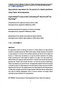
o F mg Figure 1: System of simple pendulum with all considered forces: tension force F and earth gravitational force mg.



dθ dt

2

+

F g cos θ − = 0, l ml

(2)

where string tension F and angular position θ is function of time t. The simplest way to solved Equation (2) to obtain solution of θ is by solving r dθ F g =± − cos θ dt ml l

(3)

numerically with some initial conditions. Equation (3) is a little bit different than that is proposed in [9] which is r dθ 2g =± (cos θ − cos θ0 ), dt l

(4)

with initial conditions θ(0) = +θ0 and dθ/dt(0) = 0. Equation (3) can be solved numerically. Using Euler method it can be written as

θ± (t + ∆t) = θ± (t) ±

r

F (t) g − cos θ± (t)∆t. ml l

(5)

Equation (5), for both θ± , will be tested using artificial data produced by 3

Equation (1) dan (2). Equation (1) will give the following numerical equations to produce θ(t)

g α(t) = − sin θ(t), l ω(t + ∆t) = ω(t) + α(t), θ(t + ∆t) = θ(t) + ω(t),

(6) (7) (8)

with initial conditions θ(t) = θ0 and ω = 0 at t = 0. The produced time series of θ(t) will be used to produce F (t) using F (t) = mlω 2 (t) + mg cos θ(t).

3

(9)

Results and discussion

The θ(t) has been simulated with l = 1 m, g = 10 m/s2 , θ0 = 0.5236 rad, ω0 = 0, tmax = 10 s, ∆t = 10−3 s, and m = 0.2 kg. Using this time series the value of ω(t) is calculated using

ω(t) =

θ(t) − θ(t − ∆t ), ∆t

(10)

and then the string tension F (t) is calculated using Equation (9), (10), and the time series θ(t). Figure 2 shows the result of simulated θ(t) and the string force F (t) produced from the θ(t) is given in Figure 3. Time series of F (t) has periode double than the time series of θ(t). At time t about 0.5 s the pendulum bob passes a point where it has minimum height. This point, also at t about 1.5, 2.5, and other similar points, divide the range of one oscillation periode into two identical region where value of the string tension in these two regions with the same |θ| has the same value. That is way the periode of string tension F (t) has periode double than the θ(t). In this model only magnitude of F (t) 4

0.6

θ (rad)

0.4 0.2 0 -0.2 -0.4 -0.6 0

1

2

3

4

5 6 t (s)

7

8

9 10

Figure 2: Produced times series θ(t) with l = 1 m, g = 10 m/s2 , θ0 = 0.5236 rad, ω0 = 0, tmax = 10 s, and ∆t = 10−3 s. is calculated that the direction always point to a point where the system is hung. The mathematical explanation is simpler, Equation (9) gives always positive value from θ(t): the ω 2 (t) and cos[θ(t)]. Unfortunately, direct application of Equation (5) to calculate θ(t) from F (t) give unintepreted results which has no physical meaning since value of θ(t) can be more than ±2π rad. This result is shown in Figure 4. This could be lied on the ± sign in right side of Equation (5). Further investigation shows that the calculated θ(t) does not produce the same F (t) when it is used to calculate F (t) using Equation (9). It means that the integration used in this report does not guarantee that the results are self consistent. The different between F (t) and F [θ(t)] which is represented as ∆F is given in Figure 5. A correction must be applied to overcome this problem. An algorithm that could reduce the value of ∆F could probably give the right θ(t). This is the explanation why the previous result of θ(t) could have such a large value θ ∈ [−6 : 6] rad even the initial angle only 0.5236 rad. An iteratif self consisten field scheme is used to overcome this obstacle, but unfortunately can not handle this problem. Other way is to modify Equation (5) by notifying the behaviours of F (t) and θ(t) from Figure 2 and 3. Then Equation (5) is modified into 5

2.6

F (N)

2.4 2.2 2 1.8 1.6 0

1

2

3

4

5 6 t (s)

7

8

9 10

Figure 3: Produced times series F (t) with l = 1 m, g = 10 m/s2 , m = 0.2 kg and ∆t = 10−3 s from previous θ(t).

|F (t + ∆t) − F (t)| θ(t + ∆t) = θ(t) − F (t + ∆t) − F (t)

r

F (t) g − cos θ(t)∆t. ml l

(11)

This modification can be implemented since the time series of F (t) is already available. The result is given in Figure 6. The difference between θ(t) and calculated θcalc (t), which is produced from F (t), is defined as ∆θ = |θ(t)| − θcalc (t).

(12)

Plot of ∆θ against t is given in Figure 7.

4

Conclusion

A numerical procedure to obtain time series of angular displacement θ(t) from string tension time series F (t) of a simple pendulum has been reported. 6

6

θcalc (rad)

4 2 0 -2 -4 -6 0

1

2

3

t (s)

Figure 4: Produced times series θ(t) from F (t) in Figure 3 for: θ+ (◦) and θ− (2). The similar Form of the equation that holds for tangential direction must be treated differently for radial direction since there is a quadratic term that hides the information of direction of angular velocity. A modification to the reqular form is shown and proved that it works. Only one minor problem remains, that the produced angular displacement has only positive values. The difference between orignal and reproduced angular displacement is below 0.04 rad for initial angular displacement 0.5236, or about 7.6 % error.

Acknowledgements Authors would like to thank to Research Division Research Grant from Institut Teknologi Bandung, Indonesia, in 2011 for partially support this work.

References [1] Paolo Palmieri. A phenomenology of galileo’s experiments with pendulums. The British Journal for the History of Science, 42:479–513, 2009. 7

4

∆F (N)

3 2 1 0 0

1

2

3

t (s)

Figure 5: The difference between F (t) and F [θ(t)] for: θ+ (◦) and θ− (2). [2] Douglas C. Giancoli. Physics for Scientists and Engineers with Modern Physics. Pearson Education International, fourth edition, 2009. [3] Harris Benson. University Physics. John Wiley & Sons, Inc., revised edition, 1996. [4] David Halliday, Robert Resnick, and Jearl Walker. Fundamentals of Physics. Wiley-India, sixth, extended edition, 2006. [5] A. Bel´endez, A. Hern´andez, A. M´arquez, T. Bel´endez, and C. Neipp. Analytical approximations for the period of a nonlinear pendulum. European Journal of Physics, 27(3):539, 2006. [6] R. Cuerno, A. F. Ran ada, and J. J. Ruiz-Lorenzo. Deterministic chaos in the elastic pendulum: A simple laboratory for nonlinear dynamics. American Journal of Physics, 60(1):73–79, 1992. [7] John M. Schmitt and Philip V. Bayly. Bifurcations in the mean angle of a horizontally shaken pendulum: Analysis and experiment. Nonlinear Dynamics, 15(1):1–14, 1998. [8] Ernest L. Edwardes. Huygens, christiaan (1658). horologium. the hague: Adrian vlaqc. Antiquarian Horology, 7(1), 1970.

8

0.6

θcalc (rad)

0.4 0.2 0 -0.2 -0.4 -0.6 0

1

2

3

4

5 6 t (s)

7

8

9 10

Figure 6: Produced θcalc (t) from F (t) in Figure 3. [9] F. M. S. Lima and P. Arun. An accurate formula for the period of a simple pendulum oscillating beyond the small angle regime. American Journal of Physics, 74(10):892, 2006. [10] Claudio G. Carvalhaes and Patrick Suppes. Approximation for the period of the simple pendulum based on the arithmetic-geometric mean. American Journal of Physics, 76(12):1150–1154, 2008. [11] Richard B. Kidd and Stuart L. Fogg. A simple formula for the largeangle pendulum period. The Physics Teacher, 40(2):81–83, 2002. [12] Khusnul Khotimah. Pengaruh panjang tali, sudut awal, dan massa bandul terhadap periode serta menentukan konstanta redaman pada ayunan sederhana, Master thesis, Institut Teknologi Bandung, 2011. [13] Unknown. The not so simple pendulum, URI http://www2.yk.psu. edu/~kxt7/Labs/Hasan/Pendulum.pdf [20110706 13.02]. [14] Siti Nurul Khotimah, Sparisoma Viridi, Novitrian, Mitra Djamal, and Rachmat Hidayat. Measuring system of simple pendulum tension to obtain motion of pendulum bob. The 2nd International Conference on Instrumentation, Communications, Information Technology, and Biomedical Engineering (ICICI-BME) 2011, 2011 (submitted).

9

0.01

∆θ (rad)

0 -0.01 -0.02 -0.03 0

1

2

3

4

5 6 t (s)

7

8

9 10

Figure 7: The difference between θ(t) and calculated θcalc (t).

10