A Simple, Practical Distributed Multi-Path Routing ... - CiteSeerX

A Simple, Practical Distributed Multi-Path Routing Algorithm Johnny Chen and Peter Druschel and Devika Subramanian Department of Computer Science Rice University November 18, 1998

Abstract

We present a simple and practical distributed routing algorithm based on backward learning. The algorithm periodically oods scout packets that explore paths to a destination in reverse. Scout packets are small and of xed size; therefore, they lend themselves to hop-by-hop piggy-backing on data packets, largely defraying their cost to the network. The correctness of the proposed algorithm is analytically veri ed. Our algorithm also has loop-free multi-path routing capabilities, providing increased network utilization and route stability. The Scout algorithm requires very little state and computation in the routers, and can eciently and gracefully handle high rates of change in the network's topology and link costs. An extensive simulation study shows that the proposed algorithm is competitive with link-state and distance vector algorithms, particularly in highly dynamic networks.

1 Introduction We introduce a simple distributed routing algorithm that is based on the idea of backward learning [1]. The key idea underlying this algorithm is the periodic ooding of small, xed sized messages through the network, which explore available paths to a destination1 . These exploratory messages, called Scouts, are of a xed, small size, and can be readily piggy-backed onto data packets on a hop-by-hop basis. This largely defrays their cost to the network. The algorithm is comparable in simplicity to the conventional link-state (LS) algorithm. However, Scout requires far less state and computation in the routers, and is comparable to the distance-vector (DV) algorithm in this respect. Unlike LS and DV, Scout's routing trac requirements do not vary with the network's rate of change in topology or trac conditions. To achieve a comparable rate of route convergence, Scout's routing trac requirements exceed that of LS and DV by a small factor under low rates of network change, but match those of LS and DV under highly dynamic network conditions. Scout can easily be extended to compute multiple path between each source and destination, and to forward packets loop-free along the computed paths. Multi-path routing can aord greater utilization of available network resources, and avoids routing oscillations in 1

In general a destination could represent a single host, a subnetwork, or an entire routing domain.

1

networks with dynamic (i.e., trac-dependent) route cost metrics. The Scout algorithm is particularly attractive in networks that are highly dynamic and where routers are resource constraint. Such conditions arise in mobile, wireless networks and personal communications systems (PCS). The rest of this paper is organized as follows. In Section 2, we describe the proposed algorithm and present an analysis of its convergence properties. We then describe a simple multi-path extension to the algorithm that guarantees loop freedom. In Section 4, we present an extensive comparative simulation study focusing on speed of convergence both during initial route discovery and in response to topology changes (link failures and subsequent recovery), end-to-end delivery delay and bandwidth, routing trac, and robustness in the event of router state corruption. We show comparative results evaluating the LS, DV, and our proposed algorithm on multiple network topologies, ranging from a simple, illustrative topology to larger networks that resemble the structure of the Internet inter-domain topology. We conclude with a discussion of related work and future directions in Sections 5 { 7.

2 Scout Routing Algorithm There are two key conceptual ideas underlying our algorithm: ecient, self-stabilizing shortest paths and loop-free multi-path routing. In this section, we describe these concepts in the context of the single path Scout algorithm (SP Scout) and provide extensions to nd multiple paths in Section 3.

2.1 Flood Based Route Discovery We proceed by initially assuming idealized network characteristics and then progressively remove these assumptions and present additions to the algorithm that deal with the relaxed assumptions. A proof of correctness and convergence under the generalized conditions is presented later in this section. Ideal Network: To feature the basic concepts of the algorithm, we assume  Static network topology where all links have unit cost.  Message delay along each link is equal. We de ne the shortest-path tree rooted at node R as a tree which connects all reachable nodes to R with the least cost. The basic mechanism of route discovery is through message ooding. In the Scout algorithm, each node in the network periodically sends a Scout message to all its neighboring nodes. Let R be the node initiating the Scout message. The period between two consecutive

oodings of Scout messages from R is called the broadcast interval (BI). A Scout [R, CR ] contains the originating node's address, R, and the cost to reach R, CR. Initially CR is zero. When a node P receives a Scout message [R, CR] from its neighbor Q, P rst modi es the Scout's cost CR to include the cost of sending a message from P to Q, C 0R = CR + Cost(P ! Q). C 0 R 2

represents the cost a message will take if it is sent by P via Q to R. Under the two assumptions above, if P has already seen a Scout from R in the current broadcast interval, P already has a route to R with cost at least C 0R . In this case, P remembers this alternate path but does not forward the Scout. Otherwise [R,CR] is the rst Scout P has seen in this broadcast interval, then P forwards [R, C 0R ] to all its neighbors except Q. Since nodes only forward R's Scout at most once in each BI, the ooding of Scout messages terminates after every node has forwarded a Scout message of the form [R, CR ]. This means the total number of Scouts exchanged in each broadcast interval for a single node is O(L), where L is the number of links in the network. After the termination of R's BI, every node in the network knows the minimum path to R. This knowledge is represented in the form of a next-hop address: node P knows the minimal path to R if P knows the minimal cost to R and which of its adjacent nodes is on the minimal path. In the Scout algorithm, node P knows the shortest cost to R and the shortest next-hop to R when P receives the rst Scout message in a BI. Nodes decide the shortest next-hop to R as the neighbor from whom they received the least cost Scout in the current BI. The forwarding tree constructed is a sink tree rooted at R. Since nodes only advertise (or forward) the least cost route to R, the Scout algorithm guarantees that all nodes will know the minimum path to R when ooding terminates. All pairs shortest path is computed once every node in the network oods its Scout message; thus the worst case time complexity of the Scout algorithm is O(NL) messages, where N is the number of nodes in the network. To disambiguate Scout messages from one broadcast interval with another, we assume for the time being that before R oods, all messages of R's previous ood are terminated. This requires the BI to be at least the time it takes for a message to traverse the longest path in the network. We remove this assumption in our general algorithm. N1: [N1, 0]

N10

N2

N2: [N1, 1]

N3: [N1, 1]

N4: [N1, 1]

N6 N8

N3

N10: [N1, 3] N3: [N1, 3]

N7 N4

N5

N6: [N1, 2]

N9

N8: [N1, 4]

N6: [N1, 2]

N7: [N1, 2]

N5: [N1, 2]

N8: [N1, 3] N5: [N1, 3] N9: [N1, 3] N7: [N1, 3]

N9: [N1, 4] N10: [N1, 4]

N8: [N1, 4]

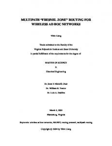
Figure 1 Example network topology and the rst round broadcast tree from N1. All link costs in the network are 1.

Figure 1 shows the broadcast tree for Scout message ooding initiated by N1 in the above network under our idealized assumptions. A broadcast tree represents an event ordering of sending and receiving messages. The gure illustrates a sequence of events in which Scouts are sent and received after N1 initiates a broadcast interval. A node Ni: [Nx, k] in the tree represents an event in which 3

Time

N1

node Ni receives a Scout [Nx, CN0 x] . Edges show Scout message transmissions and time ows downward in the gure. For events on the same level of the tree, we adopt the convention that events on the left happen earlier than events on the right. For example, event N6: [N1,2], the child of N2: [N1,1] happens before N6: [N1,2], the child of N3: [N1,1]. That is, node N6 receives a Scout from N2 before receiving one from N3, therefore as the gure shows, N6: [N1,2] child of N2: [N1,1] forwards the Scout while the other does not. Leafs of the tree correspond to events which occurred on nodes who have already received a Scout from N1. As Figure 1 shows, the shortest path is computed when ooding terminates. Non-uniform link cost and delay: The algorithm above relies heavily on the assumption that the rst Scout message of a BI is the one with minimal cost. Next, we remove this assumption by allowing non-unit link costs and non-uniform (but bounded) link delays. We preserve the assumption that all Scouts of R are terminated before R's next ood and that the network topology is static. We de ne two terms. Node P's designated neighbor to R in the broadcast interval i is de ned as the neighbor that gave P the least cost Scout to R in broadcast interval i ? 1. P's upstream node to R in broadcast interval i is the neighbor which provided the Scout that P forwarded to its neighbors (after modifying its cost). As with the previous algorithm, every node R periodically oods its Scout message [R, CR]. Upon receiving [R, CR] from a neighbor, P computes C 0R as before. In the rst broadcast interval, immediately after receiving the rst Scout message from R, node P forwards [R,C 0R ] to all neighbors except R. Node P might receive more of R's Scouts in the same BI, indicating dierent paths and path costs to R. P remembers these Scouts and adjusts its data forwarding table to re ect the new paths, but P does not forward the Scout messages. In the next broadcast interval, P waits to receive a Scout message from its designated neighbor before

ooding. When P receives the Scout from this designated neighbor, P computes C 0 R and examines all other Scout messages it has received in the current BI (including the one from its designated neighbor), to nd the Scout with the least cost C 00R to R2 . P forwards [R, C 00R ] to all neighbors except the neighbor from which it received the Scout with the least cost. This neighbor is now P's upstream node for this BI. As an example, consider the network in Figure 1 with the cost of edge (N1, N2) and (N1, N3) set to 5 and all other edge weights being 1. In the rst broadcast interval of N1, the broadcast tree is exactly the same as in Figure 1, except the cost of the N2 and N3 subtree is increased by 4. Figure 2 shows the broadcast tree for the second broadcast interval of N1. Notice in Figure 2, N7 does not forward the rst Scout it receives (one from N3) but waits for N5 (its designated neighbor) and then forwards the Scout with the least cost. The shortest-path tree is computed in the third broadcast interval when N3, N8 and N9 wait for N7 and forward the least cost Scouts to N6 and N10. In general, with a dynamic network, the least cost Scout may not come from the designated neighbor, since link costs may change between broadcast intervals.

2

4

N1: [N1, 0] N2: [N1, 5]

N3: [N1, 5]

N6: [N1, 6]

N6: [N1, 6] N7: [N1, 6]

N10: [N1, 7] N3: [N1, 7]

N3: [N1, 4]

N9: [N1, 9]

N5: [N1, 2]

N7 waits for N5

N8: [N1, 8] N7: [N1, 9]

N4: [N1, 1]

N7: [N1, 3] N8: [N1, 4]

N3, N8, N9 will wait for N7 in the next broadcast interval

N9: [N1, 4] N8: [N1, 5]

Figure 2 Broadcast tree after the second round of ooding from N1 in the network of Figure 1 with unequal link costs.

Under these network assumptions, the shortest path computation to any node R is bounded by K broadcast intervals, where K is the depth of the shortest-path tree rooted at R. In the example above, the depth of the shortest-path tree is 5 and the Scout algorithm converged in 3 broadcast intervals. It is worth mentioning that although the shortest-path computation is bounded by K broadcast intervals, all nodes know a path to R after R's rst broadcast interval. The quality of the path progressively improves with additional broadcast intervals. Unrestricted Network: We can remove the remaining network assumptions with the following algorithmic changes which do not aect the time to compute shortest paths3 . The static network assumption guarantees that if node P receives a Scout message in the previous broadcast interval from neighbor Q, P will also receive a Scout message from Q in the current broadcast interval. If links are allowed to fail and recover, P might never receive another message from Q. We modify the algorithm by requiring P to ood the rst Scout message from R if P did not ood any of R's Scout messages in the previous BI. In other words, if P waited for a Scout from its designated neighbor Q in the previous BI but never received a Scout, instead of waiting for Q, or any other neighbor in the current round, P immediately

oods the rst Scout it sees in the current broadcast interval and recalculates its designated neighbor. We do not allow P to wait for a neighbor in the current BI, in particular, the designated neighbor, because if there are multiple failures, waiting for the best information might cause cascading waits. Our decision was motivated by the observation that propagating more recent, perhaps sub-optimal, information is more useful than trying to wait for the best information which entails the risk of not propagating any information at all. To handle overlapping broadcast intervals from the same source, we simply add a sequence number to the Scout messages indicating the current broadcasting interval. The sequence 3

Shortest path computation time only applies when the network is not changing for some period.

5

number ensures that the algorithm only makes routing decisions based on the information from the most recent broadcasting interval. Figure 3 summarizes the general SP Scout algorithm. 1. Destinations periodically generate a Scout with an increasing sequence number. 2. On receiving a Scout, the router discards the Scout if the Scout sequence number is not current OR the Scout advertises a path to the current node. 3. The router adds the cost of the incoming link to the cost of the Scout and A. If the router has not forwarded a Scout (from the same source) in the last BI, flood the Scout. B. Else if Scout is from the designated neighbor, forward the least cost Scout (from the same source) received in the current BI. C. Else store the Scout. 4. Update forwarding table to reflect the shortest path.

Figure 3 SP Scout Algorithm Summary for Unrestricted Networks

2.2 SP Scout Proof of Correctness We prove the shortest path convergence time for the unrestricted Scout algorithm by showing that sink trees rooted at R are iteratively transformed into shortest-path trees rooted at R in a number of rounds bounded by the structure of the network. Intuitively this follows because every node eventually receives a Scout from the neighbor with the lowest cost to R, and therefore every node eventually knows the shortest path to R. We de ne SPT as the shortest-path tree rooted at R. SPT has depth K , and SPTi as the subtree of SPT , also rooted at R, such the depth of SPTi is i. Ti is the sink tree built from R's broadcast tree built by the Scout algorithm in broadcast interval i. Tree A contains tree B i B is a subtree of A and A and B share the same root. We prove that 8i 2 [0; : : :; K ], Ti contains SPTi . Lemma 1: Assuming Ti contains SPTi , then for all nodes P 2 Ti \ SPTi, P will not change its forwarding tables in subsequent trees Tj ; j > i. Proof: Since node P 2 SPTi , P already has the shortest path (in cost and next-hop) to the sink R. Thus in subsequent broadcast rounds of R, P cannot receive a Scout with a lower cost, in fact, P will always receive the same lowest cost from the same neighbor (its designated neighbor). Therefore P will not alter its forwarding table (both cost and next-hop) in subsequent broadcast rounds. This implies nodes of distance i or less from the root R in Ti will stay in the same position in Ti+1. Theorem: Broadcast tree containment: 8i 2 [0; : : :; K ], SPTi is contained in Ti . Proof: by induction on the depth of the broadcast tree Ti. 6

Base: i = 0. SPT0 = R, and the root of T0 is R by de nition of sink trees, therefore T0 contains SPT0. Induction: Assume 8w < z < K; Tw contains SPTw , proof that Tz+1 also contains SPTz+1 . Let the set mz = leaf nodes of(SPTi). By the induction hypothesis and the algorithm structure, the set of nodes mz know that in round z + 1, they should wait for their parent node in Tz , who will oer them the shortest cost to R. Thus in broadcast interval z +1, nodes in mz forward only R's least cost Scout to their neighbors. This implies neighbors of node n 2 mz are guaranteed to receive n's shortest path to R. In particular, leaf nodes L = leaf nodes of(SPTz+1 ) will receive the minimal path cost from nodes in mz . After the broadcast interval z + 1, nodes l 2 L deduces the minimal path to R is through its parent node in mz (by the de nition of SPTz+1 ). So the leaf nodes of Tz+1 are attached in to the same nodes in SPTz+1 . And from lemma 1, interior nodes in Tz+1 preserve the same connections as nodes in Tz ; Therefore, Tz+1 contains SPTz+1 . From the induction when z = K ? 1, TK will contains SPTK , and SPTK = SPT . Since SPT contains all nodes in the network, by the tree containment de nition, TK must equal SPT . Thus after K broadcast rounds of R, the Scout algorithm is guaranteed to have computed the shortest path to R. When z > K , Tz obviously contains SPT from lemma 1. Intuitively, non-uniform link costs and link delays cause the Scout algorithm more broadcast intervals to convergence because a link can advertise a high cost in the reverse direction (to R) but have very fast forward propagation (away from R). When this occurs, node P will initially ood the costly Scout. The extra number of broadcast intervals needed to send the minimal cost Scout to P is exactly the shortest distance (in links) from P to an ancestor of P on the shortest-path tree who currently knows the minimal cost to R, which is always bounded by K . Theorem: Shortest Path Convergence. The unrestricted SP Scout algorithm in Figure 3 computes the single shortest path between every pair of nodes in the network. Proof: This follows directly from the theorem above. We proved that the broadcast tree eventually contains the shortest path tree for any given node sending Scouts. Thus when every node in the network generates Scouts, then in a bounded number of rounds, every node will know the shortest path to every other node. Theorem: Scout message bound on convergence. The unrestricted SP Scout algorithm in Figure 3 converges to the single shortest path on O(K ) BI's, with no more than O(L) messages per round per node. Where L is the number of links in the network. Proof: The rst bound on the number of BI's for shortest path convergence is proven above. The second follows directly from the algorithm. Since every nodes can only forward one Scout per round, at most O(L) Scouts can be forwarded per round per node.

7

3 Loop-Free Multi-path Routing The main challenge in distributed multi-path routing is not the computation of multiple paths, but the forwarding of data on those paths. Routers sending data along a speci c path must communicate to every intermediate router on the chosen path that this data is to take that speci c path. That is, routers must agree to a path assignment convention such that data are forwarded on the correct path. This agreement is implicit in single shortest path routing for two reasons: 1) because router only has one path to a destination, there is no ambiguity on which path to use to reach a given destination. 2) Shortest paths have the property that if the shortest path from node N1 to Nm is (N1; N2; : : :; Nm), then Ni's shortest path to Nm must be (Ni; : : :; Nm), 8i; 1  i < m. Thus, the agreement between routers to forward data on the shortest path requires 1) all routers compute the shortest path (this is built in the routing algorithm) and 2) data be tagged with its destination address. Unfortunately, this path agreement is not implicit in multi-path routing; neither of the reasons that allow implicit agreement in single shortest path is true in multiple paths. First, if node N1 computes a path (N1; N2; : : :; Nm) to Nm , it is not guaranteed that 8i; 1 < i < m, Ni will compute the path (Ni; : : :; Nm). Second, even if the correct paths are computed by all intermediate routers, the intermediate routers must decide correctly on which path to forward a particular packet, since they might have multiple path to Nm .

3.1 Scout Multi-path Extension In this section, we extend the Scout algorithm to loop-free multi-path routing. We call this algorithm the MP Scout algorithm. The approach we adapt to the router agreement problem is to tag data packets with a path ID. Path IDs are created by Scouts and provide path agreement among routers. To do this, we add a eld to a Scout packet indicating the ID of the path it is creating. The criteria for discarding and forwarding Scouts ensures loop free paths. Multipath ID. To route packets using multiple paths, there must exist a mechanism by which intermediate routers know on which path (given the router has multiple paths to the packet's destination) to forward packets they receive. Our solution is to use path IDs: each distinct path to a destination has a dierent ID, and packets traversing that path carry that path's ID. This way, a router knows how to forward packets based on a packet's destination-ID pair. To ensure loop-freedom, a router needs to be able to detect when a path forms a loop. More speci cally, a router must be able to deduce from a path ID whether the path speci ed by the ID traverses itself more than once. To this end, we construct hierarchical path IDs so that routers can quickly determine loop freedom of a path. Our IDs are represented by a xed length sequence of integers, x1 :x2:::xn , where xi = 0 indicates the eld is unused. In our implementation, the IDs are 64-bits long and are divided into 16 4-bit integer slots 8

Scout Forwarding and ID Creation. We modify the Scout algorithm slightly to per-

form loop-free multipath. First, each Scout packet carries a path ID in addition to the source, cost, and sequence number. When router R generates a Scout [R, CR, SeqNo, ID], R sends a Scout with a dierent ID to each of its neighbors by modifying the rst eld of the ID such that they are distinct4 . When a router P receives a Scout [R, CR, SeqNo, X ] from neighbor Q, P checks if it has already seen a Scout with ID Y from R with the same sequence number such that Y is a pre x of X : we say that ID A is a pre x of ID B if A = a1:a2 ::::an and B = b1 :b2:::bn+k where k > 0, and 8i; 1  i  n, ai = bi. If P has seen such a path, P concludes that this new path traverses P more than once, constituting a loop and discards the Scout. Otherwise, if the Scout that P receives from Q has the right sequence number, P computes CR0 as before and stores the path in its routing table. Next, P forwards this Scout, with the added cost and modi ed path ID, to all of its neighbors except Q. P modi es the Scout's path ID as follows: for each neighbor Qi , P assigns to the next unused ID slot (xk ) a unique non-zero number. In our example, P forwards to neighbors Qi a Scout of the form [R, CR0 , SeqNo, x1 :::xk?1:i:xk+1:::xn], where 8j > k; xj = 0.5 MP Scout Thresholding. To make the mangement of various path IDs ecient, we limit the number of paths a router may store to a destination to K , where K is some integer. A router replaces a path with a new path if the old path has a higher cost than the new one. This guarantees that in steady state, the multipath version of the Scout routing algorithms will generate no more than K Scout per destination. Using this thresholding, routers calculate the K best path to all destinations, where \best" is de ned by the cost metric. The K thresholding may be wasteful because it might propagate paths (Scouts) that are signi cantly inferior and therefore never used. To eliminate this waste, we introduce a data threshold. P keeps and forwards Scouts if the Scout's advertised cost is less than the data threshold, which is a percentage of the least cost path to the same destination seen for that round. That is, P discards Scouts advertising costs to a destination that are greater than the data threshold (eg. 20%) of the minimal cost known thus far to the destination. Notice the algorithm still waits for its designated neighbor and oods only on receiving a Scout from that neighbor. Thus in steady state, the data threshold is applied with respect to the best cost to any destination. Packet Forwarding. Each data packet in the network carries an additional path ID eld. When a host generates a packet destined for Dst, it chooses, according to some distribution, a path from the set of paths it knows to Dst and assigns the chosen path's ID to the packet. Whenever a router P receives a packet destined for Dst with a non-zero ID, P matches all the paths it knows to nd a path ID such that it is a pre x of the packet's path ID. If such We show later that distinctness is not necessary for correctness. It only enhances better multipath route generation If there are more neighbors than there are bits to encode them (in an ID slot), P wraps the IDs. Also if there are no slots left in the ID, P simply oods the Scout with the ID unmodi ed. We show that these two boundary cases only aect the number of mult-paths the MP Scout algorithm is able to nd, but do NOT aect the correctness of the algorithm. 4

5

9

an path ID is found, this P forwards the packet according to that path's speci ed next-hop neighbor. Notice at most one path ID can possibly match. An ID might not match because the path was discarded by P either because of the thresholding or because that path no longer exist (eg. link failures). If there does not exist such a path ID, then P changes the packet's ID to the minimal cost ID and forwards the packet on the minimal path. router 1

N2

30

2

N4

1

path ID next-Hop 1 2.2 2.3.1 2 1.2 1.3.2

N1 N4 N3 N1 N2 N3

N3 2

2

30

N4

1

1

N1

N2

1

2

1

Node

3

1 3

Cost

Node

30 31 32 30 31 32

N3

path ID next-Hop 1.3 2.3 1.2.3 2.2.3

N2 N4 N4 N2

Cost 31 31 32 32

Figure 4 Simple example network and forwarding table entries to N1. In the network, the numbers above the links are costs and numbers in boxes are link port numbers with respect to that router. The table below shows forwarding tables for routers N2-N4 to N1. N1:[N1, 0, X, 0] N4: [N1, 30, X, 2]

N2: [N1, 30, X, 1] N4: [N1, 31, X, 1.2]

N3: [N1, 32, X, 1.2.3]

N2: [N1, 33, X, 1.2.3.1]

N3: [N1, 31, X, 1.3]

N1: [N1, 32, X, 1.2.1]

N4: [N1, 32, X, 1.3.2]

N3: [N1, 31, X, 2.3]

N2: [N1, 31, X, 2.2]

N2: [N1, 32, X, N1: [N1, 32, X, 2.3.1] 2.2.1]

N1: [N1, 33, X, N2: [N1, 33, X, 1.3.2.1] 1.3.2.2]

N1: [N1, 33, X, 2.3.1.1]

N4: [N1, 33, X, 2.3.1.2]

N3: [N1, 32, X, 2.2.3]

N4: [N1, 33, X, 2.2.3.2]

Figure 5 First round broadcast tree for MP Scout based on network in previous Figure Example. As an example, consider the network shown in Figure 4. The numbers above

the edges represent the cost of traversing the link.6 The numbers in boxes next to the nodes represent the link port numbers with respect to that node; we use these port numbers to generate path IDs. The table below shows each node's routing table to N1 after a Scout broadcast interval7 . Figure 5 shows MP Scout's broadcast tree initiated at N1. The last eld

For simplicity, link costs in this network are symmetric. The MP Scout algorithm works correctly with asymmetric link costs. 7 The probability eld of the routing table is not shown.

6

10

in the Scout is the path ID and the sequence number is X . The data threshold in this example is 10%. Scouts are forwarded as before, with the addition of their path IDs. When a Scout is forwarded, the next unused ID eld is set to the port number on which that Scout is forwarded. For example, when N1 initially sends Scouts to N2 and N4, the IDs are 1 and 2 corresponding to N1's outgoing port number. In this example all Scouts at the leaf nodes are discarded because they advertise looping paths. Consider node N2 when it receives the Scout [N1, 33, X, 1:2:3:1], depicted by the node N2:[N1, 33, X, 1:2:3:1]. This Scout is discarded because N2 has already seen a Scout, [N1, 30, X, 1], whose ID is a pre x of the one just received. Note that that path ID 1:2:3:1 represents the path (N2,N3,N4,N2), which contains a loop. From the tables in the bottom of Figure 4, nodes N2 and N4 know of three paths to N1 and N3 knows of 4 paths. If N3 wishes to send a packet to N1, it picks from the set of known paths and picks one, say 1:2:3. N3 forwards this packet according to the chosen path's next hop, N4. When N4 receives this packet, it nds a path ID which is a pre x of the packet's path ID. There is only one that matches, the path ID 1:2; N4 forwards the packet to N2. Similarly, N2 only has one ID that matches (path ID 1), N2 then forwards the packet to N1. The broadcast from N1 took 18 messages. The number of Scouts forwarded is directly related to the number of paths one wishes to discover; we later present experimental results to quantify the tradeo between Scout trac and the number of alternate paths discovered. The broadcast initiated by N3 only requires 8 Scouts to be forwarded, the same number sent by SP Scout. This is because MP Scouts carrying alternate paths are all discarded by the data threshold, therefore nodes only forward one Scout per BI. Figure 6 summarizes the MP Scout algorithm.

3.2 MP Scout Correctness In this section, we present intuitive arguments to show that MP Scout algorithm calculates loop-free paths. Recall that loop freedom is determined by the path IDs. Thus to show that paths are loop free, we need to show that path ID generation and discarding policies guarantee loop-free paths. Scout path IDs are covered by three cases:

 Normal ID assignment. A router receives a Scout with its ID having at least one unused

eld, and each of the router's out-going links can be uniquely encoded in an ID eld.  A router has too many out-going links and cannot uniquely encode them in one ID eld.  The Scout received does not have any unused ID elds.

Proposition: MP Scout loop freedom. The MP Scout algorithm summarized in Figure 6

computes loop-free paths under normal ID assignment. Reason: Assume there exist a path  with ID X such that  is a looping path. This implies there must exist a router P such that  traverses P more than once. If  passes P 11

1. Destinations periodically generate a Scout with an increasing sequence number and proper path ID. 2. On receiving a Scout, a router discards the Scout if the Scout advertises a path that passes through itself (via prefix matching). OR sequence number is not current. 3. The router adds the cost of the incoming link to the cost of the Scout and A. If the router has not forwarded a Scout (from the same source) in the last BI, flood the Scout. B. Else if Scout is from the designated neighbor, forward the least cost Scout received in the current BI (from the same source) . Then forward Scouts it has stored which satisfy the data threshold with respect to the least cost Scout. C. Else if the router has already received the Scout from its designated neighbor for this BI and this new Scout is within the data threshold, forward this Scout. D. Else, store this Scout. 4. When forwarding Scouts, the router assigns Scout path IDs in the previously described hierarchical manner. 5. Update forwarding table to reflect known paths.

Figure 6 MP Scout Algorithm Summary for Unrestricted Networks more than once, then the Scout that carried path  also passes P more than once. That is, P accepted a path carried by a Scout it previously forwarded. Assume Scout B advertises path with ID Y is modi ed and forwarded by P and later returns as Scout A advertising path  with ID X . When P receives Scout A, P will discard this Scout for two reasons. 1) ID pre x: if the path is in P's routing table, then ID Y will be a pre x of ID X . 2) Path cost: If path was replaced by another path (ie. a better path), then path  cannot be better than because link costs are positive and  includes . This means P will also discard Scout A. Therefore a router never accepts Scouts it has already seen and forward, so looping paths can never be calculated. Proposition: The MP Scout algorithm computes loop-free paths under conditions where there are no unused ID elds and/or individual ID elds not large enough to distinguish all out-going links of a router. Reason: In the rst case, when a router receives a Scout without any unused ID eld, the router forwards the Scout as usual leaving the ID unmodi ed. In the second case, if a router has too many out-going links such that it cannot be uniquely encoded in an ID eld, the router simply \wraps" the out-going ID assignment. That is, some out-going links are not uniquely identi ed in an ID eld. We want to show that loop-freedom is still preserved under these circumstances. The proof is straight forward because the loop-freedom argument above still holds. The pre x matching still prevents looping paths because when the ID elds are exhausted because identical IDs are pre xes of themselves, so pre x matching is sucient to detect loops. 12

In the case where there are not enough bits allocated in an ID eld to distinguish all of a router's out-going links, the loop-free argument again holds. In this scenario, paths that do not form loops may be falsely matched and thus discarded. This case might discards more paths than if there had been enough bits to encode the out-going links, but never admits more paths. In both of these cases, not being able to distinguish that two IDs in fact represent dierent paths, the MP Scout algorithm may potentially discard more paths than if it could distinguish them. However, the algorithm, under these two \boundary" conditions, never admits more paths, thus loop freedom is still preserved.

3.3 Calculating Multiple Paths Multi-path routing has many advantages over single path routing, ranging from increased bandwidth to reducing route oscillation and better network load balance. The type of multiple paths one wish to calculate depends on the objective of the network. One objective could be to increase bandwidth and load balance, then the algorithm presented earlier for calculating paths subject to thresholding may be sucient. If the objective is to increase bandwidth and reliability, then calculating disjoint paths may be the desired path property. Here, we show how node and link disjoint paths can be calculated using MP Scout. Node disjoint paths: each router, in addition to running the base MP Scout algorithm, does the following: 1. Each router only forwards one Scout per destination. 2. If a router knows more than one path to a destination, it sends its second best path to its designated neighbor for that destination. 3. On receiving multiple paths to the same destination, router must make sure that the path IDs have no common pre xes. That is, the rst element in the path IDs must dier8 . Link disjoint paths can be calculated by modifying the rst condition. Instead of requiring routers to only forward one Scout, we allow routers to forward one Scout per link, where the Scouts forwarded on each out-going link could advertise dierent paths. Figure 7 illustrates the paths calculated by each algorithm. The two main paths to node A are depicted by dotted lines. In the node disjoint paths, node D knows two paths to A, (D; B; A) and (D; C; A). In this example, node D forwarded the Scout received from C (the thin line). This is why E knows path (E; D; C; A), F knows (F; D; C; A), and B knows (B; D; C; A). D also forwarded another path (advertised by B ) to its designated neighbor C (by rule 2), thus C knows two node disjoint paths to A, (C; A) and (C; D; B; A). 8

Full Path IDs (ie. no more entries left in the ID eld) are assumed to pre x match all other IDs.

13

Node Disjoint Paths

Link Disjoint Paths

A

B

A

C

B

D

E

C

D

E

F

F

Figure 7 Node and link disjoint path calculation. The paths to node A in each network are constructed either as node or link disjoint paths. The thick and thin dotted lines show the paths each node has to A. In the link disjoint example, notice that D forwarded a dierent Scout on each of its outgoing links. For out-going links (D; B ) and (D; E ), D forwarded the Scout from B , and for links (D; F ) and (D; C ) , D forwarded the Scout from C . This results in E knowing the path (E; D; B; A) and F knowing path (F; D; B; A).

3.4 MP and SP Scout Comparison Figures 6 and 3 summarizes the SP Scout and MP Scout algorithm. The main dierences between the two algorithms are 1) routers in the MP Scout algorithm are allowed to forward more than one Scout per BI and 2) Scouts carry an hierarchical path ID. Forwarding more than one Scout per BI means the MP Scout algorithm typically generates more routing trac than SP Scout. The consequence is that the MP Scout will converge to the shortest path faster and nd multiple routes. This tradeo between more routing trac and faster convergence multiple paths is quanti ed in the experimental section. The second major dierence is the path ID. This addition makes the MP Scout message double in size compared to the SP Scout. However, this ID is essential to providing loop freedom and correct packet forwarding. It is worth mentioning that the MP Scout algorithm is in some sense a generalization of the SP Scout algorithm. For example, consider the MP Scout algorithm when the data threshold is 0%, then steady state behavior (in number of Scouts and Scout traversal) of the two algorithms are exactly the same.

3.5 LS and DV Discussion The Scout algorithm diers from traditional routing algorithms in three aspects  Resource consumption 14

 Information propagation  the ability to multipath Resource consumption is measured as the amount of routing resources, memory, CPU cycles, etc., and network resources is measured by number of messages and size of the messages. The Scout algorithm has low memory requirements, similar to the Distance Vector (DV) algorithm, where all information stored by routers is contained in the routing table. This is in contrast with the Link State algorithm (LS), where each node (router) stores the complete network topology and computes the shortest-path tree. LS uses the knowledge of the entire network to eciently propagate topology or link changes and alter global routing decisions. In networks with low topological or link metric changes, our algorithm requires more network resources than both DV and LS because it maintains very little state in the router and does not exchange local topology information, relying instead on Scouts to explore paths in the network. However, in networks with high rates of changes, the Scout algorithm generates similar routing trac than DV or LS (see Section 4.2.3). In addition, since Scout messages are small and xed length, they can be piggybacked onto data packets which helps defray their cost. In the area of information propagation, the Scout algorithm is similar to LS. Both algorithms only propagate the most recent information know thus far and are not susceptible to propagating \stale information". The Scout algorithms use and forward only information carried by the Scout with the highest sequence number and LS broadcasts only the most recent local topologies. DV advertises information under the assumption that they are still valid; this allows the algorithm to globally adapt to local topology changes. However, if the assumed information is actually incorrect, routing loops and count-to-in nity could occur. In both the DV and LS algorithms, any node in the network is capable of altering global routing decisions. This makes the algorithms more adaptive because nodes with knowledge of local changes in network characteristics can proactively disseminate the information throughout the network. The Scout algorithm is unable to make use of such local information; however, this is also one of the reasons the Scout algorithm is very resilient to state corruption. Scout broadcast intervals can be shortened to increase response time to network changes. We examine these issues empirically in Section 4. One of the main features of our Scout algorithm is its ability to naturally compute loopfree multi-path routes. Our algorithm achieves this by simply assigning IDs to dierent paths leading to the same destination. It is not as easy to modify DV or LS to compute multiple loop-free paths. Extending DV to perform multipath routing would signi cantly increase the size of distance vector packets; moreover, the impact of problems such as count-to-in nity in a multi-path environment is unclear. The major obstacle of extending LS is the assignment of path IDs. In addition to calculating multiple path, all nodes must have global consensus on the paths and the IDs for those paths. 15

4 Experimental Results In this section, we present the results of extensive simulations that were performed to evaluate the proposed Scout algorithms, and to compare its behavior with that of the distance-vector (DV) and link-state (LS) routing algorithms. The algorithms are evaluated on networks with a simple illustrative topology, and more realistic topologies derived from a subset of the Internet inter-domain topology. The simulation environment is based on the \x-netsim" package from the University of Arizona [2], an execution-driven, packet-level network simulator. The simulator takes as input a description of the network topology, including link characteristics such as bandwidth and propagation delay, and a set of software modules that implement the various protocols running on the routers and hosts of the network. Simulation time advances according to the calculated transmission and propagation delay of packets in the network. Software processing in the routers and hosts are assumed to have zero cost. Four routing protocols were implemented in the simulation testbed. The rst two are the proposed SP and MP Scout algorithms. Third, a distance-vector protocol similar to the Internet RIP protocol [4] was implemented9 . Lastly, the link-state algorithm was implemented, which is used for instance in the Internet OSPF [3] routing protocol. Both the link-state and the distance-vector protocol transmit routing information in response to state changes (triggered updates). In addition, in the DV protocol, neighboring routers exchange information every 30 seconds. In the LS protocol, routers broadcast linkstate packets every 30 minutes; for our simulations, this means that with the exception of the initial LS broadcast, only triggered broadcasts occur. In the LS and DV protocols, neighboring routers exchange Hello messages to monitor the state of links. A Hello message is exchanged once per second. If a router does not see four consecutive Hello messages, it assumes the associated link has failed. However, a single Hello message is sucient to convince a router that a failed link has recovered.

4.1 Simple Topology We rst study the Scout algorithms under the simple topology depicted in Figure 8. This topology was chosen to demonstrate the key features of the various routing algorithms. In this network each link has an associated scalar value shown in the gure, which represents the cost of crossing the link. In this network, all nodes are routers and destinations. Simulations were run for 25 seconds of simulated time. This time was chosen such that each routing protocol can reach steady state conditions between successive changes in the state of the network. At time t = 0s, the network is started with initial conditions. The link connecting N1 and N4 fails at time t = 7s, and it recovers at time t = 15s. The Scout algorithm uses a broadcast interval of 2 seconds, starting at t = 0s, and a data threshold of 10%. That is, trac is 9

Our implementation includes the \split horizon" and \poison reverse" heuristics.

16

N2

9

N1

N10

1

1

N3

6

1

N6

1

9

2

1

1

N7 N4

1

N5

1

N8

1

N9

Figure 8 Example Network Topology forwarded only on paths with a cost that is within 10% of the best path's cost. Note that the failures and recoveries occur between oodings.

4.1.1 Packet Delay The rst experiment quanti es end-to-end delivery latency, which is an important aspect of a routing algorithm's performance as perceived by a network application. Figures 9 and 10 show the end-to-end delivery delay, in number of network hops, measured during the simulation described above10. In the plot, each diamond represents one packet transmission. Starting at t = 1s, host N10 sends messages to N1 at a rate of 670 messages per second. This rate is low enough to ensure that no queuing occurs in the network. Therefore, congestion cannot arise, and delivery delay directly re ects the quality of the paths chosen by the routing algorithm. The gures show the results for the Scouts, DV, and LS protocols, respectively. A reported delay of zero hops means that the packet was lost, i.e., it was never delivered to its destination. MP Scout Algorithm 8

7

7

6

6

Number of Hops

Number of Hops

SP Scout Algorithm 8

5 4 3 2 1

5 4 3 2 1

0

0 0

5

10 15 Time (secs)

20

25

0

5

10 15 Time (secs)

20

25

Figure 9 Packet delay: MP Scout and SP Scout To a rst approximation, all algorithms achieve the shortest path N10-N8-N7-N5-N4-N1 (5 hops, cost=10) during periods when the link N1-N4 is available, and N10-N6-Nf3,2g-N1 10

It is assumed here that each link has unit delay.

17

Link State 8

7

7

6

6

Number of Hops

Number of Hops

Distance Vector 8

5 4 3 2 1

5 4 3 2 1

0

0 0

5

10 15 Time (secs)

20

25

0

5

10 15 Time (secs)

20

25

Figure 10 Packet delay: Distance Vector and Link State (3 hops, cost=11) otherwise. Notice the SP Scout took two BIs to converge to the least cost path whereas the MP Scout converged in only one BI. This is because routers can forward more than one MP Scouts per BI. MP Scout splits trac among multiple paths: when the link N1-N4 is up, 35% of the packets take the 5 hop path with cost 10, and 32% are routed via the two 3 hop paths of cost 11. Splitting trac in this way can lead to an increase in available bandwidth, but this cannot be observed in the delay plots. Experiments showing the available bandwidth are presented later in this section. In response to the failure of the shortest path link N1-N4 at t = 7s, packets are lost for a period of 0{2 seconds with Scout, and 4{5 seconds with LS and DV, depending on the relative timing of the failure with respect to the periodic Scout ood or Hello message transmission. Both SP and MP Scout adjusted to the failure after one broadcast interval because N10 only received Scouts from N6 in that round. After the recovery, it took the SP Scout 3 BIs to adjust to the new shortest path: in the rst BI after recovery, the route to N1 using link (N1,N4) was known to N4 and N5. The second BI, N7 is aware of the route AFTER forwarding the path via N3's. Finally in the third round, N7 waits for N5 and forwards the optimal information. In contrast, it only took MP Scout one ood to adjust to the new shortest path and redistribute trac accordingly. MP Scout adapts quicker because the MP Scout algorithm allows routers to forward more than one Scout per round. Thus, MP Scout is guaranteed to nd the shortest path in one broadcast round after recovery. LS and DV can adjust to the new shortest path upon receiving the rst Hello message across N1-N4, 0{1 seconds after the recovery. Single diamonds represent packets that are rerouted in transit. The Hello message rate and the broadcast interval were intentionally chosen to achieve a roughly comparable response time to topology changes with each algorithm. This was done to allow a meaningful comparison of routing trac generated by each algorithm.

18

4.1.2 Global Route Quality The delay plots show the quality of routes chosen between N10 and N1 only. To quantify the overall quality of routes with the Scouts during the simulation, Figure 11 shows the percentage of routing table entries (across all routers) that did not have optimal next hops, as a function of time. A value at time t is representative of the state of the aggregate routing table after the ood round at time t. MP Scout Percent Sub-Optimal 35

30

30

Percentage Not Optimal

Percentage Not Optimal

SP Scout Percent Sub-Optimal 35

25 20 15 10 5 0

25 20 15 10 5 0

0

5

10 15 Time (secs)

20

25

0

5

10 15 Time (secs)

20

25

Figure 11 SP and MP Scout Suboptimal Routes The rst observation from Figure 11 is that the MP Scout algorithm converges faster or as fast as the SP Scout algorithm in all scenarios: Initial calculation, link failure, and link recovery. This re ects the tradeo between speed of convergence and the amount of routing trac. In this example, the SP Scout took three BIs to nd the initial optimal paths from every node to every other node. The MP Scout converged it after the initial ood. Immediately after the failure and recovery of link N1-N4 at time 7s and 15s respectively, 13% of routing tables are sub-optimal. This is the percentage of routes that were aected by the topology change. For the MP and SP Scout, adjustment to link failure took two BIs, the rst one decreased the percentage to 4.4% and the second to 0%. To see the 4.4% sub-optimal routes after the failure, consider node N5. During N1's rst BI after the link failure, N7 does not forward any Scouts because it is waiting for a Scout from its designated neighbor, N5. Thus during that period, N5 does not have a route to N1, therefore it is sub-optimal. Only after the second BI, when N7 realizes that it did not forward a Scout in the previous round, does N7 forward the N3's Scout (carrying the optimal path) to N5. As explained in Section 4.1.1, the SP Scout took 3 BIs to converge to the optimal routes. The MP Scout took only one BI. For the MP Scout, all routes are optimal upon the second

ood following an event. Note also that for MP Scout optimality is guaranteed after the rst

ood following a link recovery, and after the second ood following a link failure, assuming that a path exists. This is true independent of the network topology. 19

4.1.3 Cumulative Trac Figure 12 shows the amount of routing trac generated by each of the algorithms in our simulation. The cumulative number of messages and the number of bytes of routing trac are shown as functions of simulated time. Whenever a routing message traverses one link of the network, one message transmission is recorded, and the size of the message is added to the number of bytes of routing trac. In this experiment, Scout broadcasts are closely spaced in time, resulting in staircase routing trac plot, in order to show the broadcast intervals. In later experiments, individual broadcast intervals are staggered. 3000

45000 MP Scout SP Scout Distance Vector Link State

35000

2000

Number of Bytes

Number of Messages

40000

MP Scout SP Scout Distance Vector Link State

2500

1500

1000

30000 25000 20000 15000 10000

500 5000 0

0 0

5

10 15 Time (Secs)

20

25

0

5

10 15 Time (Secs)

20

25

Figure 12 Cumulative trac. The Scout broadcasts are closely spaced in time (resulting in the staircase routing trac plot) to show the broadcast intervals. In later experiments, broadcast intervals are staggered.

In this experiment, the amount of routing trac generated by the SP Scout algorithms exceeds that of LS and DV by roughly a factor of 3 in terms of messages and in data. The MP Scout exceeded LS and DV by roughly 3 and 7, respectively. In this example and for illustrative purposes, the Scout trac accumulates as a step function, re ecting the periodic

oods. In actual implementations of Scout algorithms, broadcast intervals would be staggered and the cumulative trac would roughly be a line. With LS and DV, there is an initial step, re ecting the startup trac. After that, there is a linear increase caused by the periodic Hello messages. Additional small steps at t = 12s and t = 16s are due to triggered updates. Note that all Scout messages are small and of xed size. Therefore, these messages can be piggy-backed onto data packets on a hop-by-hop basis, substantially defraying their cost to the network. With the exception of Hello messages, the messages generated by the LS and DV algorithms are larger and not of xed size; therefore, they do not lend themselves easily to piggy-backing. Since the DV and LS protocols implement triggered updates, the amount of routing trac they generate strongly depends on the frequency of change in link costs. Scout routing trac, on the other hand, does not depend on such change. In our simulation, there are only two changes in link cost (link failure and recovery), which favors LS and DV in the comparison. In the subsequent section, we will present data that quanti es the dependence 20

of routing trac on network size, topology, rate of link changes, and global route quality. The following assumptions were made in determining the number of bytes of routing trac generated by each of the algorithms. Host addresses occupy 32 bits, and path/link costs require 16 bits. A SP Scout message carries a source address, path cost, and sequence number (2 bytes), requiring 8 bytes. A MP Scout message has an additional path ID, requiring a total of 16 bytes. We generously assume that the LS and DV algorithms incorporate optimizations that avoid the transmission of routing table entries or link state information that have not changed since the last transmission. A DV forwarding table entry contains a destination address and a path cost, requiring 6 bytes. A LS link state entry consists of a neighbor router address and a link cost, also requiring 6 bytes. The HELLO messages generated by the LS and DV algorithms require 4 bytes, and they are exchanged every second. In addition to these costs, LS and DV requires a xed number of data bytes per message for header information. Since this overhead depends on details of protocol implementations and lower layer network technology, we exclude it from the calculation of routing trac.

4.1.4 MP Scout route discovery In the simple topology, the MP Scout algorithm found 23 (or 25%) more paths than the single path routing algorithms. All these extra paths are within the data threshold (10%) of their respective shortest path. So with roughly 26% more routing message than the SP Scout, the MP Scout is able to discover 25% more paths.

4.2 Scalable Internetwork The second topology we use for our experimental evaluation more closely re ects the structure of realistic data networks. The topology is based loosely on the Internet inter-domain routing topology. The network is roughly a partial 6-ary tree with some cross edges connecting nodes at the same level of the tree, or between levels that dier by one. We use graphs with 1, 2, 3, and 4 levels with a total of 7, 43, 76, and 115 nodes and 0, 10, 25 and 25 cross edges. Link costs are as follows: Lowest level (leaf) links have cost 5, highest level links have cost 1, all other tree links have cost 2. Cross links between nodes at the same level take on the cost of tree links at that level. Cross links that connect nodes at dierent levels take on the lower level's cost. For each algorithm, we measure routing trac as a function of network size and as a function of link failure rate. For the network with 79 nodes, we also show the delivery delay and the maximum loss-free packet rate achieved with each algorithm. Finally, we show the percentage of sub-optimal routes versus time, for both low and high link failure rates, and under conditions of state corruption in one of the routers.

4.2.1 79 Node Network Packet Delay. Figures 13 and 14 show the packet delivery delay for the 79 node network, 21

where one leaf node is transmitting packets to another leaf node. There are two disjoint paths available between source and destination. One path involves 3 level-3 links, including a cross link, with a cost of 15. The other path is through the root of the tree, with a cost of 16. Each path has a capacity of 10 Mbits/second. A failure of the cross edge in question occurs at t = 7s, and it recovers at t = 15s. MP Scout Algorithm 8

7

7

6

6

Number of Hops

Number of Hops

SP Scout Algorithm 8

5 4 3 2

5 4 3 2

1

1

0

0 0

5

10 15 Time (secs)

20

25

0

5

10 15 Time (secs)

20

25

Figure 13 Packet delay: MP Scout and SP Scout, 79-node Link State 8

7

7

6

6

Number of Hops

Number of Hops

Distance Vector 8

5 4 3 2 1

5 4 3 2 1

0

0 0

5

10 15 Time (secs)

20

25

0

5

10 15 Time (secs)

20

25

Figure 14 Distance Vector and Link State, 79-node Note that the speed of convergence to new shortest paths con rms exactly the results obtained with the simple topology, with the exception that the SP Scout performed as well as MP Scout in path convergence. The MP Scout algorithm once again distributes trac over both available paths according to the paths costs. In particular, 52% of packets take the path with cost 15, while 48% take the path with cost 16. Moreover, we measured the maximum loss-free packet rate for the MP Scout and the LS and DV single shortest path algorithm and found that MP Scout can sustain 2024 KB/s while LS and DV can only sustain 1200 KB/s11 . We chose to quantify the available bandwidth by way of the maximum loss free packet rate to eliminate the in uence of complex transport protocols.

11

22

This demonstrates how multi-path routing can eectively exploit the bandwidth available on multiple disjoint paths through the network. SP Scout Percent Sub-Optimal

MP Scout Percent Sub-Optimal 5 Percentage Not Optimal

30 25 20 15 10 5

4 3 2 1

0

0 0

5

10 15 Time (secs)

20

25

0

5

10 15 Time (secs)

20

25

Figure 15 MP and SP Scout Suboptimal routes, 79-node Global Route Quality. Figure 15 shows the percentage of sub-optimal routing table

entries as a function of simulation time in the 79-node network. Here, 3.5% of the routes are aected by the link failure. The MP Scout took 1 BI to adjust to link recovery and 2 BIs to adjust to the link failure: rst diminished the percentage to 0.1% and to zero after the second BI. The SP Scout took 2 BIs to adjust to both link failure and recovery. The non-zero percentage of routes which are sub-optimal between times 8-10s and 16-18s are barely visible in the graph. MP Scout route discovery. In the 79 node topology, MP Scout discovered 56% more routes than single path algorithms while using 33% more trac than the SP Scout.

4.2.2 Aggregate Trac 120

1800 1600 Number of Bytes per link per second

Number of Messages per link per second

Percentage Not Optimal

35

SPScout MPScout DV LS

100

80

60

40

20

SPScout MPScout DV LS

1400 1200 1000 800 600 400 200

0

0 0

20

40 60 80 Network Sizes (Nodes)

100

120

0

20

40 60 80 Network Sizes (Nodes)

100

120

Figure 16 Aggregate trac, scalable network Using the scalable topology described above, we evaluate the routing trac generated by each algorithm as a function of network size and as a function of rate of change in the network. 23

Figure 16 shows the aggregate routing trac per link during the 25 seconds of simulated time for the three algorithms, as a function of network size. No failures or link cost changes occur during the simulation time. All three single path algorithms generate routing trac that scales approximately linearly with the size of the network. The MP Scout is not linear because the number of extra paths being discovered is not necessarily a linear function with respect to the number of nodes. In the case of Scouts, the slope is considerably steeper than for LS and DV. This is the principal disadvantage of the Scout algorithms when compared with LS and DV. However, this fact should be seen in light of four factors. First, the absolute amount of MP Scout routing trac for a 115 node network is still modest (around 1637 Bytes/sec and 102 msgs/sec of trac are generated per link). Second, the small (16 or 8 bytes) Scout messages can be piggybacked onto data packets on a hop-by-hop basis. Third, unlike LS and DV, Scout's routing trac does not increase with the rate of change in the network (see below). Finally, the Scout algorithms have additional capabilities (multi-path and improved resilience to router state corruption) not present in LS and DV.

4.2.3 Aggregate trac and Route Quality We evaluated the impact of changes in the network (link cost changes, including failures/recoveries) on the amount of routing trac and the global quality of calculated paths in the next experiment. The experiment measures the three single path algorithms with varying number of link failures and recoveries in a 79 node network. To ensure that failures would not partition the network, only cross edges were aected by failures. The results of this experiment are also valid if only the link costs were changed since the network is never partitioned and a failed link could be represented as a link with a very high cost. Figure 17 shows the results. Quality of Routes vs. Rate of Change

Routing Traffic (Bytes) vs. Rate of Change 1000

Link State Distance Vector Single Path Scout

30

Bytes per Second per Link

Percentage Non-Optimal Routes

35

25 20 15 10

Single Path Scout Distance Vector Link State

800

600

400

200 5 0

0 0

5

10

15 20 25 30 Rate of Topology Change

35

40

0

5

10

15 20 25 30 Rate of Topology Change

35

40

Figure 17 Routing trac and route quality as a function of rate topology of change on a 79 node network. The topology changes consists of 50% link recoveries and 50% failures.

In this experiment, we made the response times comparable by increasing the SP Scout broadcast interval to 1s and decreasing the LS and DV link failure detection to 2 Hello 24

messages. That is, if a router does not get two Hello messages from a neighbor, it assumes the link has failed. The detection of link recovery remains at one Hello message, and Hello messages are transmitted in 1s intervals. The LS and DV trigger updates are capped by \hold-downs": a DV router is allowed to broadcast at most 4 times in one second, and a LS router is allowed to broadcast its local topology at most once every second. These values are chosen such that they have similar routing trac and route quality. The rst gure in Figure 17 shows that the global route quality. The percentage of nonoptimal routes is the average of all routes that are not optimal during the sampled period divided by the total number of routes. The gure shows that under high rates of change, SP Scout performs best. DV did not perform as well because hold-downs prevented the algorithm from adjusting to topological changes at its normal pace. LS's poor route quality is not due to the hold-downs, but to the LS's basic route calculation method. For a router R to compute an optimal path in LS, R needs the up-to-date LSP's from all routers along that path and there must not be any other out-of-date router LSPs not on the path which can in uence the optimal path calculation. The percentage of these conditions occurring directly re ects the quality of LS's routes. In a topology with high rates of changes, this condition becomes less frequent and the LS route quality degrades. Notice that in LS and DV, the per link routing trac increases with the number of link changes, while the Scouts routing trac remains constant. In DV, the sub-linear routing trac curve is very evident at 32 changes per second. This is due to the hold-downs. The LS trac, on the other hand, is linear. This is because in this experiment, no two link changes occurred on the same router, thus the hold-downs never took aect. We expect that if many link changes occured on the same router, then the LS route quality may degrade even further.

4.2.4 Router State Corruption The nal experiment attempts to quantify the behavior of our routing algorithms in the event of failures. Speci cally, we are interested in failure modes where a router's internal state is corrupted. This case is of practical importance, because it can occur due to hardware, software, or con guration errors; and, it cannot easily be prevented or detected, as is the case with corruption of routing packets during transit. At t = 7s in the simulation, the router at the root of the 79 node tree suers an intermittent fault that causes its routing state to be overwritten with random values. Since we are interested in evaluating the robustness of the various algorithms, rather than that of their implementation, the routing state is corrupted in such a way that its invariants are maintained. In other words, the state is overwritten with random but plausible values. It can be shown that with all four algorithms under consideration, the corrupted router eventually recovers from the state corruption it suers. With both LS and DV algorithms, the router learns its actual local topology through the periodic exchange of Hello message, after no 25

more than ve Hello message intervals. With LS, the router learns the global topology during the next periodic broadcast of link-state information. With DV, neighbor route exchanges cause router's forwarding table to converge to actual shortest paths. In the Scout algorithms, the forwarding table converges to correct values through the periodic ooding process. We are interested in comparing the algorithms with respect to (1) the speed of recovery from the state corruption, and (2) the impact on the network's end-to-end performance during the recovery period. With LS, the recovery period is bounded by the periodic link-state broadcast interval, or four times the Hello interval, whichever is larger. In practice, the broadcast interval tends to be quite long, for instance 30 minutes in the OSPF protocol. During the recovery period, the router is unable to calculate correct routes, which may result in routing loops and the associated loss of connectivity. With DV, once the router has learned its actual local topology, it will engage in an exchange with its neighbor routers, which will eventually converge to the actual shortest paths. This exchange may require a number of exchanges that is proportional to the diameter of the network, and the range of the path cost metric12 . In practice, the process can be expected to take time on the order of seconds. During the recovery period, routing loops may again exist and cause loss of connectivity. SP Scout with Corruption

MP Scout with Corruption

35 Percentage Not Optimal

Percentage Not Optimal

14 30 25 20 15 10 5 0

12 10 8 6 4 2 0

0

5

10 15 Time (secs)

20

25

0

5

10 15 Time (secs)

20

25

Figure 18 SP and MP Suboptimal routes, 79 node, corruption Figure 18 shows the percentage of routing entries with sub-optimal values as a function of time. The corruption occurs at t = 7s. The value of 2% at t = 7s indicates that all of the root's routing table entries are incorrect (78 routes). We rst consider the SP Scout behavior. The ood at t = 8s increases this gure to 9%, and the ood at t = 10s increases it further to 24%. The ood at t = 12s almost completely resolves the problem. The reason for this behavior is that the corrupted router initially has an incorrect notion of its designated neighbors. This leads to a process where in the rst round, 12

A count-to-in nity may occur in a loop of routers involving the failed router.

26

the node does not forward any Scouts; in the second round, it forwards sub-optimal Scouts; and, in the third round, it nally forwards optimal information. Note that this process always requires three broadcast intervals, independent of the topology. The MP Scout requires only two BIs. The ood at t = 8s increases this gure to 9% for the same reason as the SP Scout. However, the next ood, at t = 10s completely restores global optimal routes. The dierence in recovery time between the SP Scout and MP Scout is that MP Scout routers are allowed to forward more than one Scout per BI. Thus Scouts carrying optimal path information are forwarded in the second BI whereas SP Scout has to propagate them between successive BIs. Again, this process always requires two broadcast intervals, independent of the topology. The gures shown re ect a worst-case scenario, because the corrupted router is the root node. In comparison, with LS and DV protocols, one expects loss of connectivity (packet loss) after the router failure for a period of time ranging from seconds to minutes. This high degree of resilience of the Scout algorithms is due to the lack of \hard" routing state, and the absence of any direct exchange of topological information among routers. With LS, a router cannot calculate correct paths unless it has a correct copy of each router's linkstate. A corrupted router cannot obtain this information until the next periodic link-state broadcast. Moreover, the failed router may broadcast its corrupted link-state, causing all other routers to calculate incorrect routes that remain in eect until the next periodic broadcast. With DV, a failed router may disseminate incorrect information from its corrupted forwarding table. The Scout algorithms have no way of disseminating corrupt routing state.

5 Related Work Scout is loosely based on the idea of backward learning [1], but extends that algorithm significantly. Scout decouples route exploration from the transmission of data packets. As a result, route exploration to a destination does not depend on trac originating from the destination. On the other hand, Scout still leverages packet trac by piggy-backing routing information on data packets on a hop-by-hop basis. Scout explores all available paths simultaneously. As a result, it can guarantee connectivity after one broadcast interval, and shortest paths convergence is usually achieved after two broadcast intervals. Unlike the basic backward learning algorithm, Scout is capable of multipath routing. Most routing protocols in current use are based on single shortest path link-state and distance vector algorithms. The OSPF link-state routing protocol [3] can perform multi-path routing, but only when multiple equal cost shortest paths are available. A number of algorithms based on either link-state and distance vector have been proposed that nd multiple disjoint paths in a network [6, 5, 7]. These algorithms make strong assumptions about the network, such as symmetric link costs and the absence of topological changes during route computations, and it is unclear how they compare to LS and DV algorithms in terms of convergence rate and routing trac. In addition, these algorithms do not address 27

the problem of practical loop-free forwarding of data packets along multiple paths.

6 Future Work The bene ts of multi-path routing range from increases in bandwidth and network utilization, increased route stability with dynamic metrics and higher admission probability in QoS networks to multi-criteria routing applications. We are currently investigating issues of integrating routing with higher network protocol layers to achieve better end-user performance. Another research area is in the evaluation of multi-path algorithms. Just as convergence and routing trac are metrics for judging single path algorithms, similar metrics need to be designed to evaluate the quality of the paths discovered by multi-path algorithms. Issues of weighing user bene t versus network resource usage need to be considered when evaluating multi-path algorithms.

7 Conclusion This paper presents, analyses and evaluates a new, simple loop-free multi-path routing algorithm for dynamic data networks. An extensive simulation study evaluates the multi-path Scout algorithm in comparison with LS and DV on realistic network topologies. The MP Scout algorithm is very simple, it rapidly responds to topological changes in the network, it requires a modest amount of routing trac that is independent of the rate of topological change in the network, and it is highly resilient in the face of router state corruption. Moreover, Scout's routing trac takes the form of small, xed-sized messages, which lend themselves to hop-by-hop piggy-backing on data packets.

References

[1] P. Baran. On distributed communication networks. IEEE Transactions on Communication Systems, CS-12:1{9, Mar. 1964. [2] L. S. Brakmo, A. C. Bavier, and L. L. Peterson. x-Sim user's manual, 1996. http://www.cs.arizona.edu/classes/cs525/xsim/xsim.html. [3] R. Coltun. OSPF: An internet routing protocol. ConneXions, 3(8):19{25, 1989. [4] C. Hedrick. Routing information protocol, 1988. Internet Request for Comment (RFC) 1058. [5] R. Ogier and N. Shacham. A distributed algorithm for nding shortest pairs of disjoint paths. In Proceedings of IEEE INFOCOM'89, 1989. [6] D. Sidhu, R. Nair, and S. Abdallah. Finding disjoint paths in networks. In Proceedings of SIGCOMM-91, pages 43{51, 1991. [7] D. M. Topkis. A k shortest path algorithm for adaptive routing in communications networks. IEEE Transactions on Communications, 36, 1988. 28