A SIMPLE PRECONDITIONER FOR A ... - Semantic Scholar

A SIMPLE PRECONDITIONER FOR A DISCONTINUOUS GALERKIN METHOD FOR THE STOKES PROBLEM BLANCA AYUSO DE DIOS, FRANCO BREZZI, L. DONATELLA MARINI, JINCHAO XU, AND LUDMIL ZIKATANOV Abstract. In this paper we construct Discontinuous Galerkin approximations of the Stokes problem where the velocity field is H(div, Ω)-conforming. This implies that the velocity solution is divergence-free in the whole domain. This property can be exploited to design a simple and effective preconditioner for the final linear system.

1. Introduction In this paper we present a preconditioning strategy for a family of discontinuous Galerkin discretizations of the Stokes problem in a domain Ω ⊂ Rd , d = 2, 3: ( −div(2νε(u)) + ∇p = f in Ω (1.1) div u = 0 in Ω where, with the usual notation, u is the velocity field, p the pressure, ν the viscosity of the fluid, and ε(u) ∈ [L2 (Ω)]d×d sym is the symmetric (linearized) strain rate tensor defined by ε(u) = 21 (∇u + (∇u)T ). The methods considered here were introduced in [40] for the Stokes problem and in [21] for the Navier-Stokes equations when pure Dirichlet boundary conditions are prescribed. In both works, the authors showed that the approximate velocity field is exactly divergencefree, namely it is H(div; Ω)-conforming and divergence-free almost everywhere. These same methods were also used in [25]. Numerical methods that perserve divergence free condition exactly are important from both practical and theoretical points of view. First of all, it means that the numerical method conserves the mass everywhere, namely, for any D ⊂ Ω we have Z u · n = 0. ∂D

As an example of its theoretical importance, the exact divergence free condition plays a crucial view for the stability of the mathematical models (see [30]) and their numerical discretizations (see [28]) for complex fluids. The focus of this paper is to develop new solvers for the resulting algebraic systems for this type of discretization by exploring the divergence-free property. In general, the numerical discretization of the Stokes problem produces algebraic linear systems of equations of the saddle-point type. Solving such algebraic linear systems has been the subject of considerable 1

2

B. AYUSO DE DIOS, F. BREZZI, L. D. MARINI, J. XU, AND L. ZIKATANOV

attention from various communities and many different approaches can be used to solve them efficiently (see [22] and references cited therein). One popular approach is to use a block diagonal preconditioner with two blocks: one containing the inverse or a preconditioner of the stiffness matrix of a vector Poisson discretization, and one containing the inverse of a lumped mass matrix for the pressure. This preconditioner when used in conjunction with MINRES (MINimal RESidual) leads to a solver which is uniformly convergent with respect to the mesh size. While the existing solvers such as this diagonal preconditioner can also be used for these DG methods, in this paper, we would like to explore an alternative approach by taking the advantage of the divergence-free property. Our new approach reduces the solution of the Stokes systems (which is indefinite) to the solution of several Poisson equations (which are symmetric positive definite) by using auxiliary space preconditioning techniques, which we hope would open new doors for the design of algebraic solvers for PDE systems that involve subsystems that are related to Stokes operator. In [21, 40] the classical Stokes operator is considered for the special case of purely homogeneous Dirichlet boundary conditions (no-slip Dirichlet’s condition). While this special case is theoretically important, it does not model well most of the cases that occur in the engineering applications (for instance, it is not realistic in applications in immiscible two-phase flows, aeronautics, in weather forecasts or in hemodynamics). For the pure homogenous no-slip Dirichlet boundary conditions, we have the following identity Z Z ε(u) : ε(v) = ∇u : ∇v. Ω

Ω

when u and v vanish on the boundary of Ω. This identity can be used when deriving the variational formulation, thus leading to simplifications of the analysis in the details related to the Korn’s inequality on the discrete level. To extend the results in [21, 40] to this different boundary condition we provide detailed analysis showing that the resulting DG-H(div; Ω)-conforming methods are stable and converge with optimal order. Furthermore, a key feature of the DG-H(div; Ω)-conforming schemes of providing a divergence-free velocity approximation is satisfied as in [21, 40], by the appropriate choice of the discretization spaces. This property is fully exploited in designing and constructing efficient preconditioners and we reduce the solution of the Stokes problem to the solution of a “second-order” problem in the space curl H01 (Ω). We propose then a preconditioner for the solution of the corresponding problem in curl H01 (Ω). This is done by means of the fictitious space [33, 34] (or auxiliary space [41, 35]) framework. The proposed preconditioner amounts to the solution of one vector and two scalar Laplacians. The solution of such systems can then be efficiently computed with classical approaches, for instance the Geometric Multigrid (GMG) or Algebraic Multigrid (AMG) methods. Throughout the paper, we use the standard notation for Sobolev spaces [1]. For a bounded domain D ⊂ Rd , we denote by H m (D) the L2 -Sobolev space of order m ≥ 0 and by k · km,D

DG FOR STOKES

3

and | · |m,D the usual Sobolev norm and seminorm, respectively. For m = 0, we write L2 (D) instead of H 0 (D). For a general summability index p, we also denote by W m,p (D) the usual Lp -Sobolev spaces of order m ≥ 0 with norm k · km,p,D and seminorm | · |m,p,D . By convention, we use boldface type for the vector-valued analogues: H m (D) = [H m (D)]d , likewise, we use boldface italics for the symmetric-tensor-valued analogues: Hm (D) := [H m (D)]d×d sym . H m (D)/R denotes the quotient space consisting of equivalence classes of elements of H m (D) that differ by a constant; for m = 0 the quotient space is denoted by L2 (D)/R. We indicate by L20 (D) the space of the L2 (D) functions with zero average over D (which is obviously isomorphic to L2 (D)/R). We use (· , ·)D to denote the inner product in the spaces L2 (D), L2 (D), and L2 (D). 2. Continuous Problem In this section, we discuss the well posedness of the Stokes problem which is of interest. We remark that the results in the paper are valid in two and three dimensions, although to make the presentation more transparent we focus on the two dimensional case, discussing only briefly the main changes (if any) needed to carry over the results to three dimensions. We begin by restating (for reader’s convenience) the equations already given in (1.1) with a bit more detail regarding the boundary conditions. For a simply connected polyhedral domain Ω ⊂ Rd , d = 2, 3 with boundary Γ = ∂Ω, we consider the Stokes equations for a viscous incompressible fluid: ( −div(2νε(u)) + ∇p = f in Ω (2.1) div u = 0 in Ω On the boundary Γ we impose kinematic boundary condition (2.2)

u·n=0

on Γ,

together with the natural condition on the tangential component of the normal stresses (2.3)

((2 ν ε(u) − pI)n) · t = 0

on Γ,

where I is the identity tensor. Note that as n · t ≡ 0 then (2.3) is reduced to (2.4)

(ε(u)n) · t = 0

on Γ.

When the space (2.5)

H 10,n (Ω) = {v ∈ H 1 (Ω) : v · n = 0 on Γ }

is introduced, the variational formulation of the Stokes problem reads: Find (u, p) ∈ H 10,n (Ω)× L2 (Ω)/R as the solution of: ( a(u, v) + b(v, p) = (f , v) (2.6) b(u, q) = 0

∀ v ∈ H 10,n (Ω) ∀ q ∈ L2 (Ω)/R

4


where for all u ∈ H 10,n (Ω), v ∈ H 10,n (Ω) and q ∈ L2 (Ω)/R the (bi)linear forms are defined by Z Z Z a(u, v) := 2ν ε(u) : ε(v) dx, b(v, q) := − q div v dx, (f , v) := f · v dx. Ω

Ω

Ω

For the classical mathematical treatment of the Stokes problem (where the Laplace operator is used instead of the divergence of the stress tensor ε(u)) existence and uniqueness of the solution (u, p) are very well known and have been reported with different boundary conditions in many places (see for instance [27, 38, 23, 24]). The Stokes problem considered here (2.1)-(2.2)-(2.3) has been derived and used in different applications [39, 42, 26]. For the Stokes problem with the slip boundary conditions (2.2)-(2.3), existence, uniqueness and interior regularity was first established in [37] (for even the more general linearized Navier-Stokes). The study of well-posedness and regularity up to the boundary for the solutions of this problem has received substantial attention only in very recent years. For example, analysis can be found in [10, 3] for weak and strong solutions in the H 1 (Ω) × L2 (Ω) and W 1,p (Ω) × Lp (Ω), 1 < p < ∞. In these works it is assumed that the boundary of Ω is at least of class C 1,1 (Ω) and the more general boundary condition of Navier slip-type is studied. In [4], the authors provide the analysis in the W 1,p (Ω) × Lp (Ω), 1 < p < ∞ for less regular domains. Here, for the sake of completeness, we provide a very brief outline of the proof of wellposedness of the problem, in the case Ω is a polygonal or polyhedral domain (which is the relevant case for the numerical approximation we have in mind). By introducing the operator D0 = −div : H 10,n (Ω) −→ L20 (Ω), it can be shown [14, 38] that D0 is surjective, i.e., Range(D0 ) = L20 (Ω). Therefore, the operator D0 has a continuous lifting which implies that the continuous inf-sup condition is satisfied. Hence, from the classical theory follows that to guarantee the well-posedness of the Stokes problem (2.1)-(2.2), it is enough to show that the bilinear form a(·, ·) is coercive; ie., there exists γ0 > 0 such that (2.7)

a(v, v) ≥ γ0 |v|21,Ω

∀ v ∈ H 10,n (Ω).

Once continuity is established, existence, uniqueness and a-priori estimates follow in a standard way. The proof of (2.7) requires a Korn inequality, that in general imposes some restrictions on the domain (see Remark 2.3). For the case considered in this work the needed result is contained in next Lemma: Lemma 2.1. Let Ω ⊂ Rd , d = 2, 3 be a polygonal or polyhedral domain. Then, there exists a constant CKn > 0 (depending on the domain through its diameter and shape) such that (2.8)

|v|21,Ω ≤ CKn kε(v)k20,Ω ,

∀ v ∈ H 10,n (Ω).

To prove the above Lemma, we first need the following auxiliary result

DG FOR STOKES

5

Lemma 2.2. For every polygonal or polyhedral domain Ω there exists a positive constant κ(Ω) such that (2.9)

κ(Ω)kηk20,Ω ≤ kη · nk20,∂Ω

∀η ∈ RM (Ω)

where RM (Ω) is the space of rigid motions on Ω defined by RM (Ω) = a + bx : a ∈ Rd b ∈ so(d) with so(d) denoting the set of skew-symmetric d × d matrices, d = 2, 3. Proof. To ease the presentation we provide the proof only in two dimensions. The extension to three dimensions involve only notational changes and therefeore it is ommitted. To show the lemma we observe that a polygon contains always at least two edges not belonging to the same straight line. A rigid movement whose normal component vanishes identically on those two edges is easily seen to be identically zero. This implies that for c ≡ (c1 , c2 , c3 ) ∈ R3 on the (compact) manyfold Z |(c1 − c3 x2 , c2 + c3 x1 )|2 dx = 1 Ω

the function Z (2.10)

|(c1 − c3 x2 , c2 + c3 x1 ) · n|2 ds

c→ ∂Ω

(which is obviously continuous) is never equal to zero. Hence it has a positive minimum, that equals the required κ(Ω). As a direct consequence of last Lemma, we can now provide the proof of the desired Korn inequality given in Lemma 2.1. Proof. (Proof of Lemma 2.1.) For every v ∈ H 10,n (Ω) we consider first its L2 projection v R on the space RM (Ω) of rigid motions and the projection v ⊥ := v − v R on the orthogonal subspace. As v · n = 0 on ∂Ω we obviously have (2.11)

v R · n = −v ⊥ · n.

Moreover, as v ⊥ is orthogonal to rigid motions we have (2.12)

|v ⊥ |21,Ω ≤ CK kε(v ⊥ )k20,Ω

for some constant CK (note that the rigid motions include the constants, so that Poincaré inequality also holds for v ⊥ ). On the other hand, since RM (Ω) is finite dimensional we have obviously (2.13)

|v R |21,Ω ≤ CP kv R k20,Ω

6


that using (2.9) gives |v R |21,Ω ≤

(2.14)

CP kv R · nk20,∂Ω κ(Ω)

and using also (2.11) and (2.12) 1 2 CP |v|1,Ω ≤ |v R |21,Ω + |v ⊥ |21,Ω ≤ kv R · nk20,∂Ω + |v ⊥ |21,Ω 2 κ(Ω) (2.15)

=

CP CT CP kv ⊥ · nk20,∂Ω + |v ⊥ |21,Ω ≤ |v ⊥ |21,Ω κ(Ω) κ(Ω)

≤

CT CP CK CT CP CK kε(v⊥ )k20,Ω = kε(v)k20,Ω κ(Ω) κ(Ω)

where the constant CT depends on the trace inequality on Ω. Defining now CKn = we conclude the proof.

2CT CP CK κ(Ω)

Remark 2.3. The proof of Lemma 2.1 relies on the assumption that the domain is polygonal or polyhedral. For more general smooth bounded domains, the Korn inequality (2.8) is still true, as long as the domain is assumed to be not rotationally symmetric. Otherwise a Korn inequality can be established by restricting the solution space (see [29, Appendix A] for further details).

3. Abstract setting and basic notations Let Th be a shape-regular family of partitions of Ω into triangles T in d = 2 or tetrahedra in d = 3. We denote by hT the diameter of T , and we set h = maxT ∈Th hT . We also assume that the decomposition Th is conforming in the sense that it does not contain any hanging nodes. We denote by Eh the set of all edges/faces and by Eho and Eh∂ the collection of all interior and boundary edges, respectively. For s ≥ 1, we define H s (Th ) = φ ∈ L2 (Ω) , such that φ T ∈ H s (T ),

∀ T ∈ Th ,

and their vector H s (Th ) and tensor Hs (Th ) analogues, respectively. For scalar, vector-valued, and tensor functions, we use (· , ·)Th to denote the L2 (Th )-inner product and h· , ·iEh to denote the L2 (Eh )-inner product elementwise. The vector functions are represented column-wise. We recall the definitions of the following

DG FOR STOKES

7

operators acting on vectors v ∈ H 1 (Ω) and on scalar functions φ ∈ H 1 (Ω) as div v =

d X ∂v i i=1

∂xi

T ∂v 2 ∂v 1 ∂φ ∂φ ⊥ curl v = − curl φ = ∇ φ := ,− ∂x1 ∂x2 ∂x2 ∂x1 3 T ∂v ∂v 2 ∂v 1 ∂v 3 ∂v 2 ∂v 1 curl v = ∇ × v = − , − , − ∂x2 ∂x3 ∂x3 ∂x1 ∂x1 ∂x2

(d = 2) (d = 3)

And, we recall the definitions of the spaces to be used herein: H(div; Ω) := {v ∈ L2 (Ω) : div v ∈ L2 (Ω) },

d = 2, 3,

H(curl; Ω) := {v ∈ L2 (Ω) : curl v ∈ L2 (Ω) } d = 2, H(curl; Ω) := {v ∈ L2 (Ω) : curl v ∈ L2 (Ω) } d = 3 . H 0,n (div; Ω) := {v ∈ H(div; Ω) : v · n = 0 on Γ }, H 0,t (curl; Ω) := {v ∈ H(curl; Ω) : v × n = 0 on Γ }, H 0,n (div0 ; Ω) := {v ∈ H 0,n (div; Ω) : div v = 0 in Ω }. The above spaces are Hilbert spaces with the norms kvk2H(div,Ω) := kvk20,Ω + kdiv vk20,Ω

∀ v ∈ H(div; Ω) ,

kvk2H(curl,Ω) := kvk20,Ω + kcurl vk20,Ω

∀ v ∈ H(curl; Ω).

kvk2H(curl,Ω) := kvk20,Ω + kcurl vk20,Ω

∀ v ∈ H(curl; Ω) .

Remark 3.1. It is worth noting that if we restrict our analysis to vectors u and v in H 1 (Ω) ∩ H 0,n (div0 ; Ω) then problem (2.6) becomes: Find u ∈ H 1 (Ω) ∩ H 0,n (div0 ; Ω) as the solution of: (3.1)

a(u, v) = (f , v)

∀ v ∈ H 1 (Ω) ∩ H 0,n (div0 ; Ω).

As is usual in the DG approach, we now define some trace operators. Let e ∈ Eho be an internal edge/face of Th shared by two elements T 1 and T 2 , and let n1 (n2 ) denote the unit normal on e pointing outwards from T 1 (T 2 ). For a scalar function ϕ ∈ H 1 (Th ), a vector field τ ∈ H 1 (Th ), or a tensor field τ ∈ H1 (Th ) we define the average operator in the usual way (see for instance [5]), that is, on internal edges/faces 1 {ϕ} = (ϕ1 + ϕ2 ), 2

1 {v} = (v 1 + v 2 ), 2

1 {τ } = (τ 1 + τ 2 ). 2

However, on a boundary edge/face, we take {ϕ}, {v}, and {τ } as the trace of ϕ, v, and τ ,respectively, on that edge.

8


For a scalar function ϕ ∈ H 1 (Th ), the jump operator is defined as [[ ϕ ]] = ϕ1 n1 + ϕ2 n2

on e ∈ Eho , and [[ ϕ ]] = ϕn on e ∈ Eh∂

(where obviously n is the outward unit normal), so that the jump of a scalar function is a vector in the normal direction. For a vector field v ∈ H 1 (Th ), following, for example, [6], the jump is the symmetric matrix-valued function given on e by [[v]] = v 1 n1 + v 2 n2

on e ∈ Eho , and [[v]] = v n on e ∈ Eh∂ ,

where v n = (vnT +nv T )/2 is the symmetric part of the tensor product of v and n. Hence, the jump of a vector-valued function is a symmetric tensor. If we denote by nT the outward unit normal to ∂T , it is easy to check that XZ XZ (3.2) v · nT q ds = {v} · [[ q ]] ds ∀ v ∈ H 1 (Th ) , ∀ q ∈ H 1 (Th ). T ∈Th

∂T

e∈Eh

e

Also for τ ∈ H1 (Ω) and for all v ∈ H 1 (Th ), we have XZ XZ (3.3) (τ nT ) · v ds = {τ } : [[v]] ds. T ∈Th

∂T

e∈Eh

e

3.1. Discrete Spaces: General framework. We present three choices for each of the finite element spaces V h and Qh to approximate velocity and pressure, respectively. For each choice, we also need an additional space Nh (resp. N h in d = 3) made of piecewise polynomial scalars and of piecewise polynomial vectors in three dimensions, to be used as a sort of potentials or vector potentials. We will explain the reason for doing this and the way in which to do this later on. Note, too, that we will use this space more heavily in the construction of our preconditioner. The different choices for the spaces V h , Qh , and Nh or N h rely on different choices of the local polynomial spaces R(T ), S(T ), and M(T ) or M(T ), respectively, made for each element T . Specifically, we have (3.4)

V h := {v ∈ H(div; Ω) : v|T ∈ R(T ) ∀ T ∈ Th , v · n = 0 on Γ} ,

(3.5)

Qh := q ∈ L2 (Ω)/R : q|T ∈ S(T ) ∀ T ∈ Th ,

and (3.6) (3.7)

Nh := ϕ ∈ H01 (Ω) : ϕ|T ∈ M(T ) ∀ T ∈ Th for d = 2, and N h := {v ∈ H(curl; Ω) : v|T ∈ M(T ) ∀ T ∈ Th v × n = 0 on Γ} for d = 3.

The three spaces V h , Qh , and Nh (or N h ) will always be related by this exact sequences: (3.8)

curl

div

0 −→ Nh −→ V h −→ Qh −→ 0.

DG FOR STOKES

9

in two dimensions, and curl

div

0 −→ N h −→ V h −→ Qh

(3.9)

in three dimensions. It is also necessary for each operator in (3.8) and (3.9) to have a continuous right inverse whose norm is uniformly bounded in h. For instance, it is necessary that 1 (3.10) ∃ β > 0 s.t. ∀h, ∀ q ∈ Qh ∃ v ∈ V h with: div v = q and kvk0,Ω ≤ kqk0,Ω . β Obviously, for the curl operator (in 2 and 3 dimensions) these bounded right inverses will be defined only on V h ∩ H 0,n (div0 , Ω). Remark 3.2. In all our examples, the pair (V h , Qh ) is among the classical (and very old) finite element spaces specially tailored for the approximation of the Poisson equation in mixed form. In particular, properties (3.8) and (3.10) always hold. 3.2. Examples. We now present three examples of finite element spaces that can be used in the above framework. For each example, we specify the corresponding polynomial spaces used on each element and describe the corresponding sets of degrees of freedom. We restrict our analysis to the case of triangles or tetrahedra; more general cases can also be considered when corresponding changes are made (see [19]). Let us first fix the notation concerning the spaces of polynomials. For m ≥ 0, we denote by Pm (T ) the space of polynomials defined on T of degree of at most m; the corresponding vector space is denoted by P m (T ) = (Pm (T ))2 . A polynomial of degree m ≥ 3 that vanishes throughout ∂T (hence it belongs to H01 (T )) is called a bubble (or an H-bubble) of degree m over T . The space of bubbles of degree m over T is denoted by HB m (T ). and its vectorvalued analogue by HB m (T ). We denote by Pm hom (T ) the space of homogeneous polynomials of degree m, and we denote by x⊥ the vector (−x2 , x1 ). For m ≥ 2, (3.11)

m m+1 m m+1 P+ (T ) P + (T ). m (T ) := P (T ) + HB m (T ) := P (T ) + HB

And, for m ≥ 1, we set (3.12)

BDMm (T ) := P m (T ),

RTm (T ) := P m (T ) ⊕ x Pm hom (T ).

Moreover we set, for d = 2 and m ≥ 0 (3.13)

TRm (T ) := P m (T ) ⊕ x⊥ Pm hom (T ).

and for d = 3 and m ≥ 0 (see [31]) (3.14)

NDm (T ) := P m (T ) ⊕ x ∧ P m hom (T ).

We also consider some generalized bubbles: a vector-valued polynomial of degree m ≥ 2 that belongs to H 0,n (div, T ) (hence whose normal component vanishes throughout ∂T ) is called a D-bubble of degree m over T . The space of D-bubbles of degree m over T is

10


denoted by DB m (T ). Similarly a vector valued polynomial of degree m ≥ d that belongs to H 0,t (curl, T ) (hence whose tangential components vanish all over ∂T ) is called a C-bubble of degree m over T . The space of C-bubbles of degree m over T will be denoted by CB m (T ). All the spaces used herein are well known and widely used. They are usually referred to as Brezzi-Douglas-Marini, Raviart-Thomas, and Rotated Raviart-Thomas spaces, respectively. The first example follows. 1. Raviart-Thomas For k ≥ 1, we take in each T , S(T ) = Pk (T ), and R(T ) := RTk (T ). The degrees of freedom in RTk (T ) are Z u · ne q ds ∀ e ∈ ∂T, ∀ q ∈ Pk (e), e

(3.15)

Z

∀ p ∈ Pk−1 (T ).

u · p dx T

As Qh is made of discontinuous piecewise polynomials, here and in the following examples the degrees of freedom in S(T ) can be taken in an almost arbitrary way. The corresponding pair of spaces (V h , Qh ) gives the classical Raviart-Thomas finite element approximation for second-order elliptic equations in mixed form, as introduced in [36]. It is well known and easy to check that the pair (V h , Qh ) satisfies div(V h ) = Qh

(3.16)

and that the property (3.10) is verified. We then take M(T ) := Pk+1 (T ) and M(T ) := NDk (T ) and note that o

curl(Nh ) ⊆ V h

(3.17)

curl(N h ) ⊆ V h

and that the operator curl (for d = 2 and d = 3) has a continuous right inverse uniformly o

bounded from V h ∩ H 0,n (div0 , Ω) to Nh and N h respectively; that is, ∃ C > 0 such that ∀h, ∀v h ∈ V h ∩ H 0,n (div0 , Ω) ∃ϕ ∈ Nh , such that (3.18)

curl ϕ = v h

and kϕk1,Ω ≤ C kv h k0,Ω .

2. Brezzi-Douglas-Marini: For k ≥ 1, we take S(T ) = Pk−1 (T ), and R(T ) = BDMk (T ). The degrees of freedom for BDMk (T ) are (see [9]): Z u · ne q ds ∀e ∈ ∂T, ∀ q ∈ Pk (e); e

Z (3.19)

u · v dx

∀ v ∈ TRk−2 (T ) k ≥ 2 and d = 2,

u · v dx

∀ v ∈ NDk−2 (T ) k ≥ 2 and d = 3.

T

Z T

DG FOR STOKES

11

The resulting finite element pair (V h , Qh ) is also commonly used for the approximation of second-order elliptic equations in mixed form introduced in [17] for d = 2 and in [32, 15] for d = 3. Also in this case it has been established that the pair (V h , Qh ) verifies the properties of (3.16) and (3.10). We then take M(T ) := Pk+1 (T ), and M(T ) := NDk+1 (T ) and note that (3.17) and (3.18) are also satisfied. 3. Brezzi-Douglas-Fortin-Marini: For k ≥ 1, we take S(T ) = Pk (T ) and R(T ) = BDFMk+1 (T ), which can be written as BDFMk+1 = BDMk (T ) + DB k+1 (T ). The degrees of freedom for BDFMk+1 (T ), though similar to the previous ones, are given here: Z u · ne q ds ∀e ∈ ∂T, ∀ q ∈ Pk (e); e

Z (3.20)

u · v dx

∀ v ∈ TRk−1 (T )

d = 2,

u · v dx

∀ v ∈ NDk−1 (T )

d = 3.

T

Z T

The resulting finite element pair (V h , Qh ) gives the triangular analogue of the element BDFMk introduced in [16] for the approximation of second-order elliptic equations in mixed form. It is easy to check that the pair (V h , Qh ) verifies (3.16) and (3.10). We then take M(T ) := P+ k+1 (T ) and M(T ) := NDk (T ) + CB k+1 (T ) ∩ NDk+1 (T ) and note that (3.17) and (3.18) hold. The three choices above are quite similar to each other, and the best choice among them generally depends on the problem and the way in which the discrete solution is to be used. We also use basic approximation properties: for instance, we recall that a constant C exists such that for all T ∈ Th and for all v, e.s. in H s (T ), an interpolant v I ∈ R(T ) exists such that (3.21)

kv − v I k0,T + hT |v I |1,T ≤ ChsT |v|s,T ,

s ≤ k + 1.

4. The discontinuous Galerkin H(div; Ω)-conforming method To introduce our DG-approximation, we start by defining, for any u, v ∈ H 2 (Th ) and any p, q ∈ L2 (Ω)/R, the bilinear forms Ah (u, v) = 2ν (ε(u) : ε(v))Th − h{ε(u)} : [[ v ]]iEho − h[[ u ]] : {ε(v)}iEho h i − 2ν hε(u)n, (v · n)niEh∂ + h(u · n)n, ε(v)niEh∂   Z Z (4.1) X X + 2ν  αh−1 [[ u ]] : [[ v ]] ds + αh−1 (u · n)(v · n) ds e e e∈Eho

Bh (v, q) = −(q, div v)Th

e

e∈Eh∂

e

∀ v ∈ H 2 (Th ), ∀ q ∈ L2 (Ω)/R

12


where as usual α is the penalty parameter that we assume to be positive and large enough. It is easy to check that the solution (u, p) of (2.6) verifies: ( Ah (u, v) + Bh (v, p) = (f , v) ∀ v ∈ H 2 (Th ) (4.2) Bh (u, q) = 0 ∀ q ∈ L2 (Ω)/R. For a general DG approximation, we now replace the spaces H 2 (Th ) and L2 (Ω)/R with the discrete ones X h and Qh , respectively. Following [21], we choose for (X h , Qh ) one of the pairs (V h , Qh ) of the previous examples in order to get a global divergence-free approximation. More generally, we can choose a pair (V h , Qh ) in order to find a third space Nh in such a way that (3.8), (3.16), (3.10), (3.17), and (3.18) are satisfied. This set of assumptions will come out several times in the sequel and, therefore, it is helpful to give it a special name. Definition 4.1. In the above setting, we say that the three spaces (V h , Qh , Nh ) (resp. (V h , Qh , N h )) satisfy Assumption H0 if (3.8) (resp. (3.9)), (3.16), (3.10), (3.17) and (3.18) are satisfied. We note that, according to the definition of V h , the normal component of any v ∈ V h is continuous on the internal edges and vanishes on the boundary edges. Therefore, by splitting a vector v ∈ V h into its tangential and normal components v n and v t v n := (v · n)n,

(4.3)

v t := (v · t)t ≡ v − v n ,

we have Z

[[ v n ]] : τ ds = 0 ∀ τ ∈ H1 (Th ),

∀ e ∈ Eh

(4.4)

e

implying that Z

Z (4.5)

∀ e ∈ Eh

[[ v ]] : τ ds =

[[ v t ]] : τ ds ∀ τ ∈ H1 (Th ).

e

e

The resulting approximation to (2.6), therefore, becomes: Find (uh , ph ) in V h × Qh such that ( ah (uh , v) + b(v, ph ) = (f , v) ∀v ∈ V h (4.6) b(uh , q) = 0 ∀ q ∈ Qh , where

(4.7)

ah (u, v) := 2ν (ε(u) : ε(v))Th − h{ε(u)} : [[ v t ]]iEho − h[[ ut ]] : {ε(v)}iEho Z X −1 + 2να he [[ ut ]] : [[ v t ]] ds ∀ u, v ∈ V h , e∈Eho

b(v, q) := −(q, div v)Ω

e

∀ v ∈ V h , ∀q ∈ Qh .

DG FOR STOKES

13

Consistency The consistency of the formulation (4.6) can be checked by means of the usual DG-machinery. In this case, it is sufficient to compare (4.1) and (4.7) and to observe that if (u, p) is the solution of (2.6), then Ah (u, v h ) ≡ ah (u, v h ),

Bh (v h , p) ≡ b(v h , p),

∀v h ∈ V h ⊆ H 0,n (div; Ω),

Further, it is evident that, Bh (u, qh ) ≡ b(u, qh ) for all qh ∈ Qh . Hence, as (u, p) verifies (4.2), it also verifies (4.6); that is, ( ah (u, v) + b(v, p) = (f , v) ∀v ∈ V h (4.8) b(u, q) = 0 ∀ q ∈ Qh . Thus, consistency is proved. To prove the existence and uniqueness of the solution of (4.6) and to obtain the optimal error bounds, we need to define suitable norms. We define the following semi-norms X X 2 h−1 ∀ v ∈ H 1 (Th ), k∇vk20,T , |[[ v ]]|2∗ := |v|21,h = e k[[ v ]]k0,e , e∈Eho

T ∈Th

and norms kvk2DG : = 2ν |v|21,h + 2ν |[[ v t ]]|2∗ X 2ν h2T |ε(v)|21,T |||v|||2 : = kvk2DG +

(4.9)

v ∈ H 1 (Th ), v ∈ H 2 (Th ).

T ∈Th

We also remark that the seminorms defined in (4.9) are actually norms with the additional requirement that v ∈ H 0,n (div; Ω). We also observe that when restricted to discrete functions v ∈ V h , the k · kDG -norm and the ||| · ||| are equivalent (using inverse inequality). Continuity can easily be shown for both bilinear forms: ∀ u, v ∈ H 2 (Th ),

|ah (u, v)| ≤ |||u||| |||v||| |b(v, q)| ≤ kvk1,h kqk0,Ω

∀ v ∈ H 1 (Th ), q ∈ L2 (Ω)/R .

Following [19], the existence and uniqueness of the approximate solution and optimal error bounds are guaranteed if the following two conditions are satisfied: (H1): coercivity: ∃ γ > 0 independent of the mesh size h such that (4.10)

ah (v, v) ≥ γkvk2DG

∀ v ∈ V h.

(H2): inf-sup condition: ∃ β > 0 independent of the mesh size h such that (4.11)

sup v∈V h

(div v, qh )Ω ≥ βkqh k0,Ω kvkDG

∀ qh ∈ Qh .

14


Condition (H2) is a consequence of the inf-sup condition that holds for the continuous problem (2.6): ∃ β > 0 s.t. ∀h, ∀qh ∈ Qh

∃ v ∈ H 1 (Ω) : div v = qh and kvk1,Ω ≤

1 kqh k0,Ω . β

It is well known that for all the families considered here an interpolation operator v → v I ∈ V h exists that verifies (3.21) (in particular for s = 1), and div v I = div v (= qh ). By observing that [[ v ]] = 0 on the internal edges as v ∈ H 1 (Ω), and by using the Agmon trace inequality [2] and (3.21) (for s = 1), we have (4.12)

|[[ v I ]]|2∗ :=

X

I 2 h−1 e k[[ v t ]]k0,e =

X

I 2 2 h−1 e k[[ (v − v)t ]]k0,e ≤ C |v|1,Ω .

e∈Eho

e∈Eho

Hence, again using (3.21), we deduce that kv I kDG ≤ C |v|1,Ω . Thus (4.11) is proved. In order to prove (4.10) we need to extend (2.8) from Lemma 2.1 to spaces of discontinuous vectors. We have therefore the following result. Also see Appendix A for further comments on the validity of the result in three dimensions. Lemma 4.2. Let V h be a piecewise polynomial subspace of H 0,n (div; Ω). Then, ∃ CK > 0 independent of h such that   X 2  (4.13) |v|21,h ≤ CK kε(v)k20,Th + h−1 , ∀ v ∈ V h. e k[[ v t ]]k0,e e∈Eho

Proof. To show (4.13), a direct application of [13, Inequality (1.14)] to v ∈ V h gives   Z 2 X   2 2 −1 2  he k[[ v t ]]k0,e + sup v · ηdx  (4.14) |v|1,h ≤ CK kε(v)k0,Th +  , e∈Eho

η∈L2 (Ω) R kηk0,Ω =1, Ω η=0

Ω

We now show that the last term in (4.14) can be bounded by the first two. We claim that 2

Z (4.15)

v · ηdx

sup η∈L2 (Ω) R kηk0,Ω =1, Ωη=0

Ω

X 2 ≤ C kε(v)k20,Th + h−1 k[[ v ]]k t e 0,e . e∈Eho

DG FOR STOKES

15

There are surely many ways of checking (4.15). Here, we propose one. For v ∈ V h and R η ∈ L2 (Ω) with Ω η dx = 0, we set Z v · η dx, I(v, η) := Ω

and we want to prove that 1/2 X 2 I(v, η) ≤ C kε(v)k20,Th + h−1 k[[ v ]]k kηk0,Ω t e 0,e

(4.16)

e∈Eho

that will easily give (4.15) taking the supremum with respect to η with kηk0,Ω = 1. To prove R (4.16) for every η ∈ L2 (Ω) with Ω η dx = 0, we consider the following auxiliary elasticity problem: Find χ ∈ H 10,n such that: (4.17)

∀v ∈ H 10,n .

(ε(χ), ε(v))0,Ω = (η, v)0,Ω

Thanks to (2.8) problem (4.17) has a unique solution, and we set (4.18)

τ := ε(χ).

We note that as natural boundary condition for (4.17) we easily have (τ )nt ≡ (ε(χ) · n) · t = 0

(4.19)

on Γ,

where t is any tangent unit vector to Γ. Due to well-known results on the regularity of the solutions of PDE systems on polygons, the solution τ of (4.17)-(4.18) (which, a priori, on a totally general domain would only be in (L2 (Ω))2×2 sym ) satisfies the following a priori estimate: there exists a p > 2 (depending on the geometry of Ω) and a constant Cp such that for all η ∈ L2 (Ω) the corresponding τ satisfies kτ k(Lp (Ω))2×2 + kdivτ k0,Ω ≤ Cp kηk0,Ω . sym

(4.20)

The proof of the following proposition (actually, in two or three dimensions) is given in Appendix A. Proposition 4.3. Let T be a triangle with minimum angle θ > 0, and let e be an edge of T . Then for every p > 2 and for every integer kmax , a constant Cp,θ,kmax exists such that Z p−2 −1/2 (4.21) v · (τ · n) ds ≤ Cp,θ,kmax hT kvk0,e (hT kdivτ k0,T + hT p kτ k0,p,T ) e 2 kmax for every τ ∈ (Lp (Ω))2×2 (e). sym with divergence in L (T ) and for every v ∈ P

Then we have Z I(v, η) = (4.22)

Z v · η dx = −

Ω

v · (divτ ) dx Ω

= (ε(v) : τ )Th − h[[ v t ]] : {τ }iEho

16


having taken into account that at the interelement boundaries the normal component of v is continuous and on Γ both the normal component of v and (τ )nt are zero. At this point, we can apply (4.21) to each e of the last term in (4.22). We apply the usual Cauchy-Schwarz inequality on the first term and we use instead the generalized Hölder inequality (with q = 1/2 and r = 2p/(p − 2), so that p1 + 1q + 1r = 1) on the second one. Then we obtain p−2 XZ X X −1/2 −1/2 [[ v t ]] : {τ } ds ≤ Cp,θ,kmax hT kvk0,e hT kdivτ k0,T + hT kvk0,e k hT p kτ k0,p,T e∈Eho

e

T ∈Th e∈∂T

(4.23) ≤ C|[[ v t ]]|∗ h kdivτ k0,Ω + C

X

h−1 e |[[ v t

]]|20,e

1/2 X

e∈Eho

kτ kp0,p,T (e)

e∈Eho

1/p X

p−2 r p

he

e∈Eho

≤ Ch |[[ v t ]]|∗ kdivτ k0,Ω + C |[[ v t ]]|∗ kτ k0,p,Ω µ(Ω)1/r where for each e ∈ Eho with e = ∂T + ∩ ∂T − , the set T (e) refers to T (e) := T + ∪ T − . In the second line, µ(Ω) denotes the measure of the domain Ω, whereas the constant C still depends on p, kmax and on the maximum angle in the decomposition Th . From (4.22), (4.23), and the bound (4.20) we then obtain |I(v, η)| ≤ C (kε(v)k0,Th + |[[ vt ]]|∗ ) kηk0,Ω

(4.24)

which gives (4.16). Thus the proof of the lemma is complete.

Remark 4.4. The fact that in inequality (4.13) only the jumps over the interior edges e ∈ Eho (but not on the boundary edges) are included, prevents a direct and straightforward application of the results from [12]. The proof presented here is surely too elaborate, and we believe that a simpler proof is possible. However some of the machinery used here is likely to be of use elsewhere. Therefore, we decided that it would be worthwhile to present the proof we have obtained to date. The stability of ah (·, ·) in the k · kDG -norm can now be easily checked with the usual DG machinery. We have Z {ε(v)} : [[ v t ]] ds ≤ h1/2 k{ε(v)}k0,e kh−1/2 [[ v t ]]k0,e , e

which when we proceed as in [5] (or as in (4.23) with p = 2) yields X Z (4.25) {ε(v)} : [[ v t ]] ds ≤ C|v|1,h |[[ v t ]]|∗ . e∈Eho e Using (4.25) in (4.7), we then have ah (v, v) ≥ 2νkε(v)k20,Th + 2ν αk[[ v t ]]|2∗ − 4νC|v|1,Th |[[ v t ]]|∗ .

1/r

DG FOR STOKES

17

Now using the Korn inequality (4.13) and the usual arithmetic-geometric mean inequality, we easily have a big enough α : ah (v, v) ≥ γkvk2DG

∀ v ∈ V h.

We close this section with the following theorem. Theorem 4.5. Let (V h , Qh ) be as in one of our three examples. Then problem (4.6) has a unique solution (uh , ph ) ∈ V h × Qh that verifies (4.26)

div uh = 0 in Ω.

Moreover, there exists a positive constant C, independent of h, such that for every v h ∈ V h with div v h = 0 and for every qh ∈ Qh the following estimate holds: (4.27)

ku − uh kDG ≤ C ku − v h kDG ,

kp − ph k0,Ω ≤ C (kp − qh k0,Ω + ku − v h kDG ),

with (u, p) solution of (2.6). Proof. The existence and uniqueness of the solution of (4.6) follow from (4.10)-(4.11). The divergence-free property (4.26) is implied by (3.16), which holds for all our choices of spaces. Let v h ∈ V h also be divergence-free; then we obviously have that b(v h − uh , q) = 0 for every q ∈ L2 (Ω)/R. In particular, b(v h − uh , p − ph ) = 0. Hence, from the coercivity (4.10), consistency (4.8), and continuity of ah (·, ·) we deduce immediately γkv h − uh k2DG ≤ ah (v h − uh , v h − uh ) = ah (v h − u, v h − uh ) ≤ kv h − ukDG kv h − uh kDG . On the same basis we deduce that the first estimate in (4.27) follows by triangle inequality. For every wh ∈ V h , using the consistency and continuity of ah (·, ·), we have b(wh , qh − ph ) = b(wh , qh − p) + b(wh , p − ph ) = b(wh , qh − p) − ah (u − uh , wh ) (4.28)

≤ (kqh − pk0,Ω + ku − uh kDG )kwh kDG .

By dividing (4.28) by kwh kDG and then using the inf-sup condition (4.11), we immediately deduce that βkqh − ph k0,Ω ≤ kqh − pk0,Ω + ku − uh kDG , and that the second estimate in (4.27) follows again by triangle inequality.

Remark 4.6. In the assumptions of Theorem4.5, we could obviously consider any trio of finite element spaces satisfying H0. However, for choices like RT0 , not considered in our three examples, the estimate (4.27) could be meaningless, as the term ku − v h kDG does not, in general, go to zero with h. Still, this choice could be profitably used, in some cases, as a preconditioner, as it does satisfy H0, H1, and H2.

18


5. Discrete Helmholtz decompositions In this section we provide results related to the discrete Helmholtz decomposition, introduced in Section 3 that plays a key role in the design of the preconditioner. We wish to note that Discrete Helmholtz or Hodge decompositions have been shown and used in several contexts for similar spaces but with other boundary conditions (typically, homogeneous Dirichlet) in [18, 20, 7, 8]. A nice and short proof in the language of Finite Element Exterior Calculus can be also found in [9, p. 72]. Here, together with the proof of the decomposition with our boundary conditions, we provide an estimate in the DG-norm for the components in the splitting, that will be essential in the analysis of the solver, and that, to the best of our knowledge, has not been obtained or used in any previous work. So far, we have assumed that the computational domain Ω is a polygon (or polyhedron). From now on, for the sake of simplicity, we are going to work under the stronger assumption that Ω is a convex polygon or polyhedron. As is well known, this allows the use of better regularity results, and in particular the H 2 -regularity for elliptic second-order operators. Following [19] we define the discrete gradient operator G h : Qh −→ V h as (5.1)

(G h qh , v h )0,Ω := −(qh , div v h )0,Ω

∀ vh ∈ V h.

Lemma 5.1. Assume that together the three spaces (V h , Qh , Nh ) (resp. (V h , Qh , N h )) satisfy assumption H0 (given in Definition 4.1). Then, in d = 2, for any v h ∈ V h a unique qh ∈ Qh and a unique ϕh ∈ Nh exist such that v h = G h qh + curl ϕh ,

(5.2) that is,

V h = G h (Qh ) ⊕ curl Nh . If d = 3, there exists a ψ ∈ N h such that v h = G h qh + curl ψ h ,

(5.3) and therefore

V h = G h (Qh ) ⊕ curl N h . Moreover, in both cases there exists a constant C independent of h such that the following estimate holds: kG h qh kDG ≤ Ckdiv v h k0,Ω .

(5.4)

We present the proof in two dimensions; see however Remark 5.2 after this proof, where the differences for the case d = 3 are discussed. Proof. For v h ∈ V h , consider the auxiliary problem: (5.5)

− ∆q = div v h

in Ω,

∂q = 0 on ∂Ω, ∂n

Z and

q dx = 0. Ω

DG FOR STOKES

19

Owing to the boundary conditions in V h , we have that div v h has zero mean value in Ω. Hence, problem (5.5) has a unique solution, that satisfies kqk2,Ω ≤ Creg kdiv v h k0,Ω .

(5.6) We write (5.5) in mixed form: σ = −∇q in Ω,

div σ = div v h in Ω,

σ · n = 0 on ∂Ω.

and we consider directly the approximation of the mixed formulation: Find (σ h , qh ) ∈ V h × Qh such that : ( (σ h , τ )0,Ω − (qh , div τ )0,Ω = 0 ∀ τ ∈ V h, (5.7) (div σ h , sh )0.Ω = (div v h , sh )0,Ω ∀ sh ∈ Qh . Problem (5.7) obviously has a unique solution, which moreover satisfies (5.8)

kσ − σ h k0,Ω ≤ C h |σ|1,Ω ≤ CCreg h kdiv v h k0,Ω ,

given that (5.6) was used in the last step. As both v h and σ h are in V h (and as (3.16) holds), the second equation in (5.7) directly implies that div (σ h − v h ) = 0. Hence, the exact sequence (3.8) implies that (5.9)

a unique ϕh ∈ Nh

exists such that σ h − v h = curl ϕh .

Next, by using the first equation in (5.7) and then applying definition (5.1), we deduce that (σ h , τ )0,Ω = (qh , div τ )0,Ω = −(G h qh , τ )0,Ω

∀ τ ∈ V h,

which implies σ h = −G h qh , that joined to (5.9) gives (5.2). In order to prove (5.4), we recall that (5.10)

kG h qh k2DG = kσ h k2DG = k∇σ h k20,Th + |[[ (σ h )t ]]|2∗ .

For the first term, by adding and subtracting the interpolant σ I of σ and then using inverse inequality and (3.21), we have: k∇σ h k0,Th ≤ k∇(σ h − σ I )k0,Th + k∇σ I k0,Th (5.11)

≤ Cinv h−1 kσ h − σ I k0,Th + Ck∇σk0,Th .

From triangle inequality, (5.8), and standard approximation properties (see (3.21)), we have (5.12)

k∇σ h k0,Th ≤ C kdiv v h k0,Ω .

The jump term in (5.10) is estimated similarly. First, we remark that σ = −∇q with q ∈ H 2 (Ω) so that [[ σ ]] = 0 on each e ∈ Eho , and therefore |[[ (σ h )t ]]|2∗ = |[[ (σ h )t − σ t ]]|2∗ .

20


Then, using Agmon trace inequalities (5.8) and the boundedness of σ h and σ, we have X 2 |[[ (σ h )t − σ t ]]|2∗ = h−1 e k[[ (σ h )t − σ t ]]k0,e e∈Eho

≤ Ct h−2 kσ h − σk20,Th + Ct k∇(σ h − σ)k20,Th ≤ CCreg kdiv v h k20,Ω . Thus the proof is complete.

Remark 5.2. For d = 3, instead of (5.9), the exact sequence (3.9) property implies ∃ ψh ∈ N h

such that

σ h − v h = curl ψ h .

The vector potential ψ h would be uniquely determined by adding the condition div ψ = 0. In fact, on a simply connected domain, div ψ = 0 and curl ψ = 0 together with ψ ∈ H 0,t (curl, Ω) imply ψ = 0. However, in general, the solution of div ψ = 0 and curl ψ = v h together with ψ ∈ H 0,t (curl, Ω) (which is uniquely determined) does not belong to N h . A possibility to select a vector potential ψ h in a unique way could be to compute it as the approximation to the following continuous problem: Find (ψ, θ) in H 0,t (curl; Ω) × H01 (Ω) such that (curl ψ, curl φ)Th + (∇θ, φ)Th = (v h , φ)Th

∀ φ ∈ H 0,t (curl; Ω), ∀ s ∈ H01 (Ω).

(ψ, ∇s)Th = 0 Setting

o Wh := w ∈ H01 (Ω) : w|T ∈ Pk+1 (T ) ∀ T ∈ Th , o

the discrete problem reads: Find (ψ h , θh ) ∈ N h × Wh such that (curl ψ h , curl φh )Th + (∇θh , φh )Th = (v h , φh )Th (5.13)

∀ φh ∈ N h , o

(ψ h , ∇wh )Th = 0

∀ wh ∈Wh .

Problem (5.13) has a unique solution satisfying curl ψ h = v h (from the first equation), and divψ h = 0 (from the second equation). 6. Preconditioner: Fictitious Space Lemma and Auxiliary Space Framework 6.1. Preconditioner for the semi-definite system. Assume V is a Hilbert space equipped with the norm k·kV and that A : V 7→ V 0 is a bounded linear operator. We define the bilinear form (u, v)A = hAu, vi. We say A is symmetric if the bilinear form (u, v)A is symmetric. We say that A is semipositive definite if (v, v)A ≥ 0, ∀v ∈ V

DG FOR STOKES

21

and α > 0 exists such that (v, v)A ≥ αkvk2V /N (A) ,

∀v ∈ V /N (A).

And we say that A is SPD (Symmetric Positve Definite) if it is symmetric and α > 0 exists such that (v, v)A ≥ αkvk2V , ∀v ∈ V. One useful property of symmetric semi-positive definite operators is that (6.1)

Av = 0 iff hAv, vi = 0.

A preconditioner for A is another symmetric semi-positive definite operator B : V 0 7→ V . Again, we consider the bilinear form (f, g)B = hf, Bgi. The operator BA : V 7→ V satisfies (BAu, v)A = hAv, BAui = (Au, Av)B . Lemma 6.1. If A : V 7→ V 0 and B : V 0 7→ V are both symmetric semi-positive definite such that B is positive definite on R(A), then (1) B : R(A) 7→ R(BA) is an isomorphism (with the inverse satisfying trivially that B −1 (BAv) = Av). (2) The bilinear form (·, ·)B −1 defines an inner product on R(BA). (3) The bilinear form (·, ·)A defines an inner product on R(BA). (4) BA is symmetric positive definite on R(BA) with either of the above two inner products. Proof. All these results are pretty obvious, and their proofs are similar. Let us give the proof for 3 as an example. We only need to verify that (·, ·)A is positive definite on R(BA). If v ∈ R(BA) is such that (v, v)A = 0, then, by (6.1), we have Av = 0. We write v = BAw for some w ∈ V , then ABAw = 0 and hence (Aw, Aw)B = 0. As B is positive definite on R(A), we have Aw = 0. Thus, v = ABAw = 0, as desired. For the system Au = f , we can apply the preconditioner B and the preconditioned conjugate gradient (PCG) method with respect to the inner product (·, ·)B −1 with the following convergence estimate: !k p κ(BA) − 1 ku − uk kA ≤ 2 p ku − u0 kA . κ(BA) + 1 The condition number can then be estimated by κ(BA) ≤ c1 /c0 , either where c0 (v, v)B −1 ≤ (BAv, v)B −1 ≤ c1 (v, v)B −1 ,

∀v ∈ R(BA),

22


or equivalently where c0 (w, w)B ≤ (Bw, Bw)A ≤ c1 (w, w)B ,

∀w ∈ R(A),

or where −1 −1 c−1 1 (v, v)A ≤ (B v, v) ≤ c0 (v, v)A

∀v ∈ R(BA).

6.2. Fictitious space lemma and generalizations. Let us present and prove a refined version of the Fictitious Space Lemma originally proposed by Nepomnyaschikh [33] (see also [41]). Lemma 6.2. Let V˜ and V be two Hilbert spaces, and let Π : V˜ → 7 V be a surjective map. ˜ : V˜ 0 7→ V˜ be a symmetric and positive definite operator. Then B := ΠBΠ ˜ 0 is also Let B symmetric and positive definite (here Π0 : V 0 7→ V˜ 0 is such that hΠ0 g, v˜i = hg, Π˜ v i, for all g ∈ V 0 and v˜ ∈ V˜ ). Furthermore, ˜ −1 v˜, v˜i. hB −1 v, vi = inf hB Π˜ v =v

Proof. It is obvious that B is symmetric and positive semi-definite. Note that if v ∈ V 0 is ˜ 0 v, Π0 vi = hBv, vi = 0. This means that Π0 v = 0 as B ˜ is such that hBv, vi = 0, then hBΠ SPD. Hence, v = 0 as Π0 is injective. This proves that B is positive definite. ˜ 0 B −1 v. As we obviously have Π˜ For any v˜ ∈ V˜ , let v = Π˜ v and v˜∗ = BΠ v ∗ = v, we can write v˜ = v˜∗ + w ˜ with Πw˜ = 0. Thus, ˜ −1 v˜, v˜i = inf hB ˜ −1 (˜ inf hB v ∗ + w), ˜ v˜∗ + wi ˜ Π˜ v =v

Πw=0 ˜

˜ −1 v˜∗ , v˜∗ i + inf =hB

Πw=0 ˜

−1 −1 ∗ ˜ ˜ hB w, ˜ wi ˜ + 2hB v˜ , wi ˜

From the definition of v˜∗ we have ˜ −1 v˜∗ , v˜∗ i = hB −1 v, Π˜ hB v ∗ i = hB −1 v, vi, and also ˜ 0 B −1 v, wi ˜ −1 v˜∗ , wi ˜ −1 BΠ hB ˜ = hB ˜ = hΠ0 B −1 v, wi ˜ = hB −1 v, Πwi ˜ = 0. The last two identities lead to the desired result.

Theorem 6.3. Assume that A˜ : V˜ → 7 V˜ 0 and A : V 7→ V 0 are symmetric semi-definite ˜ = N (A). Then for operators. We assume that Π : V˜ 7→ V is surjective and that Π(N (A)) ˜ : V˜ 0 7→ V˜ , we have, for B = ΠBΠ ˜ 0, any SPD operator B ˜ A). ˜ κ(BA) ≤ κ(Π)κ(B Here κ(Π) is the smallest ratio c1 /c0 that satisfies (6.2)

˜v , v˜i ≤ c−1 c−1 1 hAv, vi ≤ inf hA˜ 0 hAv, vi, Π˜ v =v

∀v ∈ R(BA).

DG FOR STOKES

23

˜ A) ˜ = b1 /b0 with b1 and b0 satisfying Proof. Denote κ(B ˜ −1 v˜, v˜) ≤ b−1 (˜ b−1 v , v˜)A˜ ≤ (B ˜)A˜ , 1 (˜ 0 v, v

˜ A). ˜ ∀˜ v ∈ R(B

By (6.2), we obtain −1 2 b−1 1 c1 kvkA ≤

inf

˜ −1 v˜, v˜) ≤ b−1 c−1 kvk2 , (B 0 0 A

˜ A) ˜ Π˜ v =v,˜ v ∈R(B

∀v ∈ R(BA).

˜ = N (A), we can prove that Π0 (R(A)) ⊂ R(A) ˜ and By the assumption that Π(N (A)) ˜ A)}. ˜ {˜ v |Π˜ v = v ∈ R(BA)} = {˜ v |Π˜ v = v ∈ R(BA), v˜ ∈ R(B By Lemma 6.2, inf

˜ −1 v˜, v˜) = inf (B ˜ −1 v˜, v˜) = (B −1 v, v), (B

˜ A) ˜ Π˜ v =v,˜ v ∈R(B

Π˜ v =v

∀v ∈ R(BA).

Therefore, −1 2 −1 −1 −1 2 b−1 1 c1 kvkA ≤ (B v, v) ≤ b0 c0 kvkA

∀v ∈ R(BA).

Theorem 6.4. Assume that the following two conditions are satisfied for Π. First, kΠ˜ v kA ≤ c1 k˜ v kA˜ ,

∀˜ v ∈ V˜ .

Second, for any v ∈ V there exists v˜ ∈ V˜ such that Π˜ v = v and k˜ v kA˜ ≤ c0 kvkA . Then κ(Π) ≤ c1 /c0 and, under the assumptions of Theorem 6.3, 2 c1 ˜ A). ˜ κ(BA) ≤ κ(B c0 Remark 6.5. In view of the application of the above results to our two dimensional case (as we shall see in the next subsection), it would have been enough to restrict ourselves to the symmetric positive definite case (instead of the semi-definite case treated in the last two subsections). However we preferred to have them in the present more general setting, as in this form they are likely to be useful in many other circumstances (starting, as natural, from the extension of the present theory to the three-dimensional case). 6.3. Application to our problem. In this section we design a simple preconditioner for the linear system resulting from the approximation of the Stokes problem (2.6) defined in (4.6)-(4.7). Note that the bilinear form ah (·, ·) defined in (4.7) provides a discretization of the vector Laplacian problem −div(2νε(u)) = f

in Ω,

u · n = 0, (ε(u) · n) · t = 0 on Γ.

24


We denote by Ah the operator associated with ah (·, ·). As the solution uh ∈ V h of (4.6) is divergence-free, the discrete Helmholtz decomposition (5.2) implies that a unique ψh ∈ Nh

exists such that uh = curl ψh .

˚ h as At this point, it is convenient to introduce the space V ˚ h := V h ∩ H 0 (div0 ; Ω). V

(6.3)

We note that as the sequence (3.8) is exact, we have ˚ h ≡ curl Nh , V

(6.4)

˚ h, and that the mapping is one-to-one. Therefore, restricting the bilinear form ah (·, ·) to V ˚h ≡ in the spirit of Remark 3.1, corresponds here to restricting the trial and test space to V ˚h curl(Nh ). The discrete problem (4.6) then reduces to the following problem: Find ψh ∈ V such that (6.5)

ah (ψh , ϕh ) = (f , ϕh )

˚h ∀ ϕh ∈ V

˚h → ˚ 0 by hAh ψh , ϕh i = ah (ψh , ϕh ), ψh , ϕh ∈ V ˚ h , we can write Defining the operator Ah : V 7 V h (6.5) as Ah ψh = fh . ˚ h . Define A˜h : V h 7→ V 0 by We now use the original space V h as the auxiliary space for V h ˜ ˜ hAh uh , vh i = ah (uh , vh ), uh , vh ∈ V h . We note that Ah is a discrete Laplacian. We assume ˜h is an optimal preconditioner for A˜h . that B We now define the operator Πh : V h −→

(6.6)

˚ h ≡ curl(Nh ) V

according to (5.2), namely Πh v h = curl ϕh . ˚ h. Note that Πh is a surjective operator and that Πh acts as the identity on the subspace V The auxiliary space preconditioner for Ah is then defined by (6.7)

˜h Π∗h . Bh = Πh B

Lemma 6.6. Assume that the spaces(V h , Qh , Nh ) satisfy assumption H0. Then Bh given ˜h is an optimal preconditioner for by (6.7) is an optimal preconditioner for Ah as long as B A˜h . Proof. Following the auxiliary space techniques (Theorem 6.4), we need to check that the following two properties are satisfied: (A1): Local Stability: there exists a positive constant C1 independent of h such that (6.8)

kΠh v h kDG ≤ C1 kv h kDG

∀ vh ∈ V h

DG FOR STOKES

25

(A2): Stable decomposition: there exists a positive constant C2 independent of h such ˚ h there exists v h ∈ V h such that Πh v h = wh and that for any wh ∈ V kv h kDG ≤ C2 kwh kDG .

(6.9)

To prove (6.8) from the Helmholtz decomposition (5.2) and the definition (6.6) of Πh , we have (6.10)

v h = G h qh + curl ϕh = G h qh + Πh v h .

Using estimate (5.4) from Lemma 5.1 and the clear fact that div v h is the trace of ε(v h ), we have (6.11)

kG h qh kDG ≤ Ckdiv v h k0,Ω ≤ Ckε(v)k0,Th ≤ Ckv h kDG .

Hence, (6.8) follows from (6.10) and (6.11): kΠh v h kDG = kv h − G h qh kDG ≤ kv h kDG + kG h qh kDG ≤ Ckv h kDG . Finally, the inequality (6.9) holds with C2 = 1 by taking v h = wh .

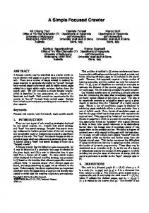
7. Numerical experiments 7.1. Setup. The tests presented in this section use discretization by the lowest order, namely, BDM1 elements paired with piece-wise constant space for the pressure. They verify the a priori estimates given in Theorem 4.5 and confirm the uniform bound on the condition number of the preconditioned system for the velocity. As previously set up, the discrete problem under consideration is given by equation (4.6) with bilinear forms ah (·, ·) and b(·, ·) defined in (4.7). In the numerical tests presented here, we take ν = 1/2 and the penalty parameter α = 6 in (4.7). We present two sets of tests

(a) Coarsest mesh

(b) Mesh for level of refinement J = 3

Figure 7.1. Meshes used in the tests for the unit square domain Ω = (0, 1) × (0, 1)

26


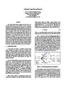
with A corresponding to the Stokes equation discretized on a sequence of successively refined unstructured meshes as shown in Figures 7.1–7.2. On the square the coarsest mesh (level of refinement J = 0) has 160 elements and 97 vertices with 448 BDM degrees of freedom. The finer triangulations of the square domain are obtained via 1, . . . , 5 regular refinements (every element divided in 4) and the finest one is with 163, 840 elements, 82, 433 vertices and 490, 496 BDM degrees of freedom. Similarly for the L-shaped domain we start with a coarsest grid (J = 0) with 64 vertices and 97 elements. For the L-shaped domain the finest grid (for J = 5) has 99, 328 elements, 50, 129 vertices and 297, 056 BDM1 degrees of freedom. In the computations, we approximate the velocity component uh of the solution of

(a) Coarsest mesh

(b) Mesh for level of refinement J = 3

Figure 7.2. Meshes used in the tests for the L-shaped domain Ω = ((0, 1) × (0, 1)) \ ([ 12 , 1) × [ 21 , 1)) the Stokes equation by solving several simpler equations (such as scalar Laplace equations). After we obtain the velocity, the pressure then is found via a postprocessing step at low computational cost. Further, for this sequence of grids the BDM1 interpolant of a function v on the k − th grid is denoted by v Ik . Accordingly the piece-wise constant, L2 -orthogonal projection of p is denoted by pIk . We also use the notation (uk , pk ) for the solution of (4.6) on the k − th grid, k = 0, . . . , 5. 7.2. Discretization error. We now present several tests related to the error estimates given in the previous sections. We computed and tabulated approximations of the order of convergence of the discrete solution in different norms. These approximations are denoted by γ0 ≈ β0 , γDG ≈ βDG , γp ≈ βp , and γ∗ ≈ β∗ . The actual orders of convergence β0 , βDG , βp , and β∗ are ku − uh k0,Ω ≈ C(u)hβ0 , kp − ph k0,Ω ≈ C(u, p)hβp ,

ku − uh kDG ≈ C(u)hβDG , |[[ uh ]]|∗ ≈ C(u)hβ∗ .

DG FOR STOKES

27

Here, as in (4.12), we denote |[[ v

]]|2∗

=

X

h−1 e

Z

[[ ut ]]2 ds.

e

e∈Eho

Note that β∗ is the order with which the jumps in the approximate solution (not in the error) go to zero. We present two sets of experiments to illustrate the results given in Theorem 4.5. First, we consider the exact given solution and calculate the right–hand side and the boundary conditions from this solution. We set (7.1)

φ = xy(1 − x)(2x − 1)(y − 1)(2y − 1),

u = curlφ.

Clearly, the function φ vanishes on the boundary of both the domains under consideration and we take u defined in (7.1) as exact solution for the velocity for both the square and the L-shaped domains. For the pressure we choose as exact solutions functions with zero mean value and select p different for the square and the L-shaped domain, namely (7.2)

p = x2 − 3y 2 + 83 xy, p = x2 − 3y 2 +

(square domain),

24 xy, 7

(L-shaped domain).

The right hand side f is calculated by plugging (u, p) defined in (7.1)–(7.2) in (2.1). Table 7.1 shows tabulation of the order of convergence of (uh , ph ) to (uI , pI ) for both the square domain and the L-shaped domain. The values approximating the order of convergence displayed in Table 7.1 are γ = log2

kuIk−1 − uk−1 k , kuIk − uk k

kpIk−1 − pk−1 k0,Ω γp = log2 , kpIk − pk k0,Ω

γ∗ = log2

|[[ uk ]]|∗ , |[[ uk−1 ]]|∗

k = 1, . . . , 5.

Here k · k stands for any of the DG or L2 norms. The quantity γ is the corresponding γ0 or γDG . From the results in this table, we can conclude that in the k · kDG norm the dominating error is the interpolation error, and as the next example shows, in general, the order of convergence in k · kDG is 1. The second test is for a fixed right hand side f = 2(1, x). We calculate approximations to the order of convergence of the numerical solutions on successively refined grids as follows: γ = log2

kuk − uk−1 k , kuk+1 − uk k

γp = log2

kpk − pk−1 k0,Ω , kpk+1 − pk k0,Ω

γ∗ = log2

|[[ uk ]]|∗ − |[[ uk−1 ]]|∗ , |[[ uk+1 ]]|∗ − |[[ uk ]]|∗

k = 1, . . . , 4.

Again, k·k denotes any of the (semi)-norms of interest and γ approximates the corresponding order of convergence. Table 7.2 shows the tabulated values of γ0 , γDG , γp , and γ∗ . It is

28


Table 7.1. Approximate order of convergence for the difference (uI − uh ) and (pI − ph ) and the jumps |[[ uh ]]|∗ for the square and L-shaped domains. Here, u and p are given in (7.1) and (7.2). Square domain k γ0

1

2

3

L-shaped domain 4

5

1.75 1.87 1.94 1.98 1.99

γDG 0.98

1.0

1.00 1.00 1.00

k γ0

1

2

3

4

5

1.69 1.79 1.90 1.96 1.98

γDG 0.97 1.01 1.01 1.00 1.00

γp

0.94 0.95 0.97 0.99 0.99

γp

0.93 0.92 0.95 0.97 0.99

γ∗

0.77 0.89 0.95 0.98 0.99

γ∗

0.73 0.85 0.93 0.97 0.99

Table 7.2. Approximate order of convergence of the error for square and Lshaped domains and right–hand side f = 2(1, x). Square domain k γ0

1

2

3

L-shaped domain 4

5

1.70 1.85 1.93 1.97 1.98

γDG 0.86 0.95 0.98 0.99 1.00

k γ0

1

2

3

4

5

1.65 1.79 1.86 1.74 1.24

γDG 0.84 0.92 0.92 0.86 0.74

γp

0.94 0.94 0.97 0.98 0.99

γp

0.91 0.89 0.88 0.82 0.70

γ∗

0.70 0.86 0.94 0.97 0.99

γ∗

0.63 0.81 0.89 0.89 0.83

clear from these values that the order of approximation for the velocity and the pressure is optimal for the square domain, whereas for the L-shaped domain the convergence is not of optimal order, due to the singularity of the solution near the reentrant corner. The numerical experiments and also the approximations for the orders of convergence presented in Table 7.1 and Table 7.2 are computed using the FEniCS package http://fenicsproject.org. 7.3. Uniform preconditioning. The tests presented in this subsection illustrate the efficient solution of the system (7.3) below by Preconditioned Conjugate Gradient (PCG) with the preconditioner given in (7.4). We introduce the matrices representing the bilinear forms defined in (4.6)–(4.7), and also the mass matrix for the BDM1 space. We denote by M the e the stiffness matrix associated with ah (·, ·) on V h in (4.6)– mass matrix on V h and by A (4.7). We note that A, without the divergence–free constraint, is spectrally equivalent to two scalar Laplacians. It is known that the null space of b(·, ·) in (4.6) is made of vector fields that are curls of continuous, piecewise quadratic functions vanishing on the boundary. We denote by Pcurl the matrix representation of these curls in the BDM space. Namely, curl(basis functions in Nh ) = (basis functions in V h )Pcurl .

DG FOR STOKES

29

It is easy to see that Aq = PTcurl MPcurl . where Aq is the discretization of the Laplacian on Nh with homogeneous Dirichlet boundary conditions. The problem of finding the solution of (6.5) then amounts to solving the following algebraic system of equations (7.3)

e curl U = PT F. PTcurl AP curl

Here the superscript T means that the adjoint is taken with respect to the `2 -inner product, U is the vector containing the velocity degrees of freedom, and F is the vector representing the right–hand side (f , v) of the problem (4.6). The matrix representation B of the preconditioner B described in the previous section has the following form: (7.4)

T −1 e −1 B = A−1 q Pcurl MA MPcurl Aq

In the numerical experiments below we have used the preconditioned conjugate gradient provided by MATLAB with the above preconditioner. We note that one may further make the ale (for A e −1 ) and Bq (for A−1 ) in (7.4). gorithm more efficient by incorporating approximations B q

In our tests the inverses needed to compute the action of the preconditoner, namely A−1 q e −1 , are calculated by the MATLAB’s backslash ”\” operator (which in turn calls the and A direct solver from UMFPACK http://www.cise.ufl.edu/research/sparse/umfpack/). The tests presented here exactly match the theory for the auxiliary space preconditioner given in Section 6.3. In summary, the action of the preconditioner requires the solution of systems corresponding to 4 scalar Laplacians. It is also worth noting that suitable multigrid packages for performing these tasks are available today. The convergence rate results are summarized in Table 7.3. The legend for the symbols used in the table is as follows: nit is the number of PCG iterations; ρ is the average reduction h i1/nit ||rnit ||`2 per one such iteration defined as ρ = ||r0 ||`2 ; J is the refinement level, for which h ≈ 2−J h0 , where h0 is the characteristic mesh size on the coarsest grid. From the results in Table 7.3, we can conclude that the preconditioner is uniform with respect to the mesh size. It is also evident that this method is in fact quite efficient in terms of the number of iterations and the reduction factor. Let us point out that when the preconditioner is implemented in 3D the action of Πh requires an implementation of the action of L2 -orthogonal (or orthogonal in equivalent inner ˚ h . This is done by solving an auxiliary product) projection on the divergence free subspace V mixed FE discretization of the Laplacian, as discussed in Section 5 and in practice it can be accomplished by considering a projection orthogonal in the inner product provided by the lumped mass matrix for BDM. In such case the solution to the auxiliary mixed FE problem

30


Table 7.3. Preconditioning results for square domain (top) and L-shaped domain (bottom). The PCG iterations are terminated when the relative residual is smaller than 10−6 . Square domain J

0

1

2

3

4

5

nit

4

4

4

5

5

4

ρ

0.016 0.023 0.031 0.034 0.033 0.031 L-shaped domain

J

0

1

2

3

4

5

nit

5

5

5

5

5

5

ρ

0.044 0.061 0.061 0.058 0.055 0.053

corresponds to a solution of a system with an M -matrix and classical AMG methods [11] AMG yield optimal solvers for such problems. The application of the preconditioner in the 3D case requires the (approximate) solution of 5 scalar Laplacians. e −1 and A−1 in (7.4) are Such extensions to 3D and also efficient approximations to A q

subject of current research and implementation and are to be included in a future release of the Fast Auxiliary Preconditioning Package http://fasp.sf.net. Appendix A. Proof of Proposition 4.3 We now state and prove a result, Proposition A.1 given below, used in Section 4 to show Korn inequality (cf. Lemma 4.2). After giving its proof, we comment briefly on how the result can be applied to show the corresponding Korn inequality (4.13) (cf. Lemma 4.2) for d = 3. Proposition A.1. Let T be a triangle (or a tetrahedron for d = 3) with minimum angle θ > 0, and let e be an edge (resp. face) of T . Then for every p > 2 and for every integer kmax there exists a constant Cp,θ,kmax such that Z d(p−2) −1/2 2p kτ k0,p,T (A.1) v · (τ · n) ds ≤ Cp,θ,kmax hT kvk0,e hT kdivτ k0,T + hT e 2 kmax for every τ ∈ (Lp (Ω))d×d (T ). sym having divergence in L and for every v ∈ P

Proof. First we go to the reference element Tˆ: Z Z Z d−1 ˆ ) dˆ ˆ ) dˆ (A.2) ˆ · (ˆ τ ·n s ≤ Cθ he v ˆ · (ˆ τ ·n s v · (τ · n) ds ≤ Cθ |e| v e

eˆ

eˆ

ˆ and τˆ are the usual covariant and contra-variant images of v and τ , respectively. where v And, here and throughout his proof, the constants Cθ and Cθ,kmax may assume different

DG FOR STOKES

31

ˆ will still be a vector-valued polynomial of degree values at different occurrences. Note that v ≤ kmax and the space H(div, T ) is effectively mapped into H(div, Tˆ) by means of the contraˆ , we construct the auxiliary function ϕv variant mapping. Then for every component vˆ of v as follows. First we define ϕv on ∂ Tˆ by setting it as equal to vˆ on eˆ and zero on the rest of ∂ Tˆ. Then we define ϕv in the interior using the harmonic extension. It is clear that ϕv will 0 belong to W 1,p (Tˆ) (remember that p > 2 so that its conjugate index p0 will be smaller than ˆ is a polynomial of degree ≤ kmax , it is not difficult to see that 2). Using the fact that v

kϕv kW 1,p0 (Tˆ) ≤ Cˆθ,kmax kˆ v k0,ê .

(A.3)

Integration by parts then gives Z Z ˆ · (ˆ ˆ ) dˆ v τ ·n s= ∂ Tˆ

eˆ

ˆ ) dˆ ϕv · (ˆ τ ·n s Z

Z = Tˆ

(A.4)

∇ϕv : τˆ dˆ x−

Tˆ

ϕv · div τˆ dˆ x

≤ |ϕv |W 1,p0 (Tˆ) kˆ τ k(Lp (Tˆ))d×d + kϕv k0,Tˆ kdiv τˆ k0,Tˆ sym ˆ ˆ k0,Tˆ ≤ C kˆ v k0,ê kˆ τ k(Lp (Tˆ))sym d×d + kϕv k0,ˆ e kdiv τ ˆ + kdiv τ k ≤ Cˆ kˆ v k0,ê kˆ τ k(Lp (Tˆ))d×d 0,Tˆ . sym

Then we recall the inverse transformations (from Tˆ to T ): − d−1 2

kˆ v k0,ê ≤ Cθ he

kvk0,e ,

−d

p , kˆ τ k(Lp (Tˆ))sym d×d ≤ Cθ h T kτ k(Lp (T ))d×d sym

2−d

kdiv τˆ k0,Tˆ ≤ Cθ hT 2 kdivτ k0,T . Inserting this into (A.4) and then in (A.2) we have then Z −d 2−d d−1 p d−1 − 2 2 kvk0,e hT kτ k(Lp (T ))d×d + hT kdivτ k0,T . v · (τ · n) ds ≤ Cp,θ,kmax he he sym e

Now we note that 1 d(p − 2) d−1 d − + =d−1− − , 2 2p 2 p and that 1 d−1 2−d − +1=d−1− + , 2 2 2 and the proof then follows immediately.

With this result in hand, we can show the Korn inequality (4.13) given in Lemma 4.2 for d = 3. It is necessary to modify the proof in only two places: the definition of the space of

32


rigid motions on Ω, RM (Ω), and the application of Proposition 4.21. The space RM (Ω) is now defined by: RM (Ω) = a + bx : a ∈ Rd b ∈ so(d) with so(d) denoting the space of the skew-symmetric d × d matrices. To prove (4.16) (and so conclude the proof of (4.13)), estimate (4.23) is replaced by estimate (A.5) below, which is obtained as follows: first, by applying (A.1) (instead of (4.21)) from Proposition A.1 to each e in the last term in (4.22) and then by using the generalized Hölder inequality with the same exponents as for d = 2 (with q = 1/2 and r = 2p/(p − 2), so that p1 + 1q + 1r = 1) XZ e∈Eho

X X

[[ v t ]] : {τ } ≤ Cp,θ,kmax

e

−1/2

hT

k[[ v t ]]k0,e hT kdivτ k0,T

T ∈Th e∈∂T

+Cp,θ,kmax

X X

−1/2

hT

d(p−2) 2p

k[[ v t ]]k0,e k hT

kτ k0,p,T

T ∈Th e∈∂T

(A.5)

≤ Ch |[[ v t ]]|∗ kdivτ k0,Ω 1/p X d(p−2) r 1/r X 1/2 X p 2 he 2p +C h−1 |[[ v ]]| kτ k t e 0,e 0,p,T (e) e∈Eho

e∈Eho

e∈Eho

≤ C|[[ v t ]]|∗ h kdivτ k0,Ω + C |[[ v t ]]|∗ kτ k0,p,Ω µ(Ω)1/r Here, as in estimate (4.23), µ(Ω) denotes the measure of the domain Ω, and the constant C still depends on p, kmax , and on the maximum angle in the decomposition Th . The rest of the proof of Lemma 4.2 proceeds as for d = 2. Acknowledgments The authors thank one of the referees for helpful comments on the first version of this work. Part of this work was completed while the first author was visiting IMATI-CNR of Pavia. She is grateful to the IMATI for the kind hospitality. The first author was partially supported by MINECO through grant MTM2011-27739-C04-04. The second and third authors were partially supported by the Italian MIUR through the project PRIN2008. The last two authors were partially supported by National Science Foundation grant DMS-1217142 and US Department of Energy grant DE-SC0009603. The authors also thank Feiteng Huang for the help with the numerical tests and in particular for putting the discretization within the FEniCS framework, and to Harbir Antil for pointing out references [10, 3]. References [1] R. A. Adams. Sobolev spaces. Academic Press [A subsidiary of Harcourt Brace Jovanovich, Publishers], New York-London, 1975. Pure and Applied Mathematics, Vol. 65.

DG FOR STOKES

33

[2] S. Agmon. Lectures on elliptic boundary value problems. Prepared for publication by B. Frank Jones, Jr. with the assistance of George W. Batten, Jr. Van Nostrand Mathematical Studies, No. 2. D. Van Nostrand Co., Inc., Princeton, N.J.-Toronto-London, 1965. [3] C. Amrouche and N. E. H. Seloula. On the Stokes equations with the Navier-type boundary conditions. Differ. Equ. Appl., 3(4):581–607, 2011. [4] H. Antil, R. H. Nochetto, and P. Sodré. The Stokes problem with slip boundary conditions on fractional Sobolev domains. (in preparation), (2013). [5] D. N. Arnold, F. Brezzi, B. Cockburn, and L. D. Marini. Unified analysis of discontinuous Galerkin methods for elliptic problems. SIAM J. Numer. Anal., 39(5):1749–1779 (electronic), 2001/02. [6] D. N. Arnold, F. Brezzi, and L. D. Marini. A family of discontinuous Galerkin finite elements for the Reissner-Mindlin plate. J. Sci. Comput., 22/23:25–45, 2005. [7] D. N. Arnold, R. S. Falk, and R. Winther. Preconditioning in H(div) and applications. Math. Comp., 66(219):957–984, 1997. [8] D. N. Arnold, R. S. Falk, and R. Winther. Multigrid in H(div) and H(curl). Numer. Math., 85(2):197– 217, 2000. [9] D. N. Arnold, R. S. Falk, and R. Winther. Finite element exterior calculus, homological techniques, and applications. Acta Numer., 15:1–155, 2006. [10] H. Beir˜ ao Da Veiga. Regularity for Stokes and generalized Stokes systems under nonhomogeneous sliptype boundary conditions. Adv. Differential Equations, 9(9-10):1079–1114, 2004. [11] A. Brandt, S. F. McCormick, and J. W. Ruge. Algebraic multigrid (AMG) for automatic multigrid solution w ith application to geodetic computations. Tech. Rep., Institute for Computational Studies, Colorado State Univ ersity, 1982. [12] S. C. Brenner. Poincaré-Friedrichs inequalities for piecewise H 1 functions. SIAM J. Numer. Anal., 41(1):306–324 (electronic), 2003. [13] S. C. Brenner. Korn’s inequalities for piecewise H 1 vector fields. Math. Comp., 73(247):1067–1087, 2004. [14] F. Brezzi. On the existence, uniqueness and approximation of saddle-point problems arising from lagrangian multipliers. Rev. Fran¸caise Automat. Informat. Recherche Opérationnelle Sér. Rouge, 8:129– 151, 1974. [15] F. Brezzi, J. Douglas, Jr., R. Dur´ an, and M. Fortin. Mixed finite elements for second order elliptic problems in three variables. Numer. Math., 51(2):237–250, 1987. [16] F. Brezzi, J. Douglas, Jr., M. Fortin, and L. D. Marini. Efficient rectangular mixed finite elements in two and three space variables. RAIRO Modél. Math. Anal. Numér., 21(4):581–604, 1987. [17] F. Brezzi, J. Douglas, Jr., and L. D. Marini. Two families of mixed finite elements for second order elliptic problems. Numer. Math., 47(2):217–235, 1985. [18] F. Brezzi and M. Fortin. Numerical approximation of Mindlin-Reissner plates. Math. Comp., 47(175):151–158, 1986. [19] F. Brezzi and M. Fortin. Mixed and hybrid finite element methods, volume 15 of Springer Series in Computational Mathematics. Springer-Verlag, New York, 1991. [20] F. Brezzi, M. Fortin, and R. Stenberg. Error analysis of mixed-interpolated elements for ReissnerMindlin plates. Math. Models Methods Appl. Sci., 1(2):125–151, 1991. [21] B. Cockburn, G. Kanschat, and D. Schötzau. A note on discontinuous Galerkin divergence-free solutions of the Navier-Stokes equations. J. Sci. Comput., 31(1-2):61–73, 2007.

34


[22] H. C. Elman, D. J. Silvester, and A. J. Wathen. Finite elements and fast iterative solvers: with applications in incompressible fluid dynamics. Numerical Mathematics and Scientific Computation. Oxford University Press, New York, 2005. [23] G. P. Galdi. An introduction to the mathematical theory of the Navier-Stokes equations. Vol. I, volume 38 of Springer Tracts in Natural Philosophy. Springer-Verlag, New York, 1994. Linearized steady problems. [24] V. Girault and P.-A. Raviart. Finite element methods for Navier-Stokes equations, volume 5 of Springer Series in Computational Mathematics. Springer-Verlag, Berlin, 1986. Theory and algorithms. [25] C. Greif, D. Li, D. Sch¨ otzau, and X. Wei. A mixed finite element method with exactly divergence-free velocities for incompressible magnetohydrodynamics. Comput. Methods Appl. Mech. Engrg., 199(4548):2840–2855, 2010. [26] G. Kanschat and B. Rivière. A strongly conservative finite element method for the coupling of Stokes and Darcy flow. J. Comput. Phys., 229(17):5933–5943, 2010. [27] O. A. Ladyzhenskaya. The mathematical theory of viscous incompressible flow. Second English edition, revised and enlarged. Translated from the Russian by Richard A. Silverman and John Chu. Mathematics and its Applications, Vol. 2. Gordon and Breach Science Publishers, New York, 1969. [28] Y.-J. Lee and J. Xu. New formulations, positivity preserving discretizations and stability analysis for non-Newtonian flow models. Comput. Methods Appl. Mech. Engrg., 195(9-12):1180–1206, 2006. [29] M. Lewicka and S. M¨ uller. The uniform Korn-Poincaré inequality in thin domains. Ann. Inst. H. Poincaré Anal. Non Linéaire, 28(3):443–469, 2011. [30] F.-H. Lin, C. Liu, and P. Zhang. On hydrodynamics of viscoelastic fluids. Communications on Pure and Applied Mathematics, 58(11):1437–1471, 2005. [31] J.-C. Nédélec. Mixed finite elements in R3 . Numer. Math., 35(3):315–341, 1980. [32] J.-C. Nédélec. A new family of mixed finite elements in R3 . Numer. Math., 50(1):57–81, 1986. [33] S. V. Nepomnyaschikh. Mesh theorems on traces, normalizations of function traces and their inversion. Soviet J. Numer. Anal. Math. Modelling, 6(3):223–242, 1991. [34] S. V. Nepomnyaschikh. Decomposition and fictitious domains methods for elliptic boundary value problems. In Fifth International Symposium on Domain Decomposition Methods for Partial Differential Equations (Norfolk, VA, 1991), pages 62–72. SIAM, Philadelphia, PA, 1992. [35] P. Oswald. Preconditioners for nonconforming discretizations. Math. Comp., 65(215):923–941, 1996. [36] P.-A. Raviart and J. M. Thomas. A mixed finite element method for 2nd order elliptic problems. In Mathematical aspects of finite element methods (Proc. Conf., Consiglio Naz. delle Ricerche (C.N.R.), Rome, 1975), pages 292–315. Lecture Notes in Math., Vol. 606. Springer, Berlin, 1977. ˇcadilov. A certain boundary value problem for the stationary system of [37] V. A. Solonnikov and V. E. Sˇ Navier-Stokes equations. Trudy Mat. Inst. Steklov., 125:196–210, 235, 1973. Boundary value problems of mathematical physics, 8. [38] R. Temam. Navier-Stokes equations, volume 2 of Studies in Mathematics and its Applications. NorthHolland Publishing Co., Amsterdam, revised edition, 1979. Theory and numerical analysis, With an appendix by F. Thomasset. [39] R. Temam and A. Miranville. Mathematical modeling in continuum mechanics. Cambridge University Press, Cambridge, 2001. [40] J. Wang and X. Ye. New finite element methods in computational fluid dynamics by H(div) elements. SIAM J. Numer. Anal., 45(3):1269–1286 (electronic), 2007.

DG FOR STOKES

35

[41] J. Xu. The auxiliary space method and optimal multigrid preconditioning techniques for unstructured grids. Computing, 56(3):215–235, 1996. International GAMM-Workshop on Multi-level Methods (Meisdorf, 1994). [42] J. Yoo, D. D. Joseph, and G. S. Beavers. Boundary conditions at a naturally impermeable wall. J. Fluid Mech., 30:197–207, 1967. ´ tica, UAB Science Faculty, 08193 Bellaterra, Barcelona, Centre de Recerca Matema Spain IUSS-Pavia c/p IMATI-CNR, Via Ferrata 5/A 27100 Pavia Italy, and Dept. of Math., KAU, PO Box 80203, Jeddah, 21589, Saudi Arabia ` di Pavia, Via Ferrata 1, 27100 Pavia, Italy Dipartimento di Matematica, Universita Department of Mathematics, Penn State University, University Park PA 16802, USA Department of Mathematics, Penn State University, University Park PA 16802, USA