Transactions of the American Fisheries Society 130:848–856, 2001 q Copyright by the American Fisheries Society 2001
A Simple Test for Nonmixing in Multiyear Tagging Studies: Application to Striped Bass Tagged in the Rappahannock River, Virginia ROBERT J. LATOUR,* JOHN M. HOENIG,
AND
JOHN E. OLNEY
Department of Fisheries Science, Virginia Institute of Marine Science, College of William and Mary, Gloucester Point, Virginia 23062, USA
KENNETH H. POLLOCK Biomathematics Graduate Program, Department of Statistics, North Carolina State University, Raleigh, North Carolina 27695, USA Abstract.—The Brownie-type models for multiyear tagging studies allow the estimation of agespecific and year-specific total survival. An important assumption of these models is that the tagged cohorts are thoroughly mixed, or more specifically, that they have identical spatial distributions. We propose a chi-square test to assess the validity of this assumption and apply the method to striped bass tagging data from the Rappahannock River, Virginia. The current protocol for estimating striped bass survival involves fitting a suite of Brownie-type models to tag recovery data. Because moderate levels of nonmixing can induce significant bias, we examined tagging data for two size ranges of fish to determine if the well-mixed assumption was violated. We suggest that examining spatial patterns of recaptures should be a routine part of analyzing tagging data from multiyear studies. For the striped bass data, the analysis showed little evidence of assumption violation, but in some cases the power of the test was probably low because the number of recaptures was small.
Brownie et al. (1985) developed a series of simple multiyear tagging models to estimate agespecific and year-specific survival and tag recovery rates. These models generalize early work by Seber (1970) and Youngs and Robson (1975) and have been applied frequently to wildlife banding studies. Recent extensions and modifications of the Brownie models have rendered this class of models more applicable to fisheries tagging studies. Pollock et al. (1991) and Hoenig et al. (1998a) showed that tag recovery rates may be converted to fishing exploitation rates when information on tag retention, tag-induced mortality, and tag reporting rate is available. Instantaneous rates of fishing and natural mortality may be determined if additional information on the seasonal distribution of fishing intensity is known at least approximately (Ricker 1975). Brownie-type models are extremely useful. An important and fundamental, but often overlooked, assumption of these models is that the cohorts of tagged animals are thoroughly mixed. Hoenig et al. (1998b) demonstrated that modest amounts of nonmixing between previously and newly tagged animals could cause serious bias and that, when
nonmixing is present, tagging data should be analyzed using models that explicitly account for nonmixing. Hoenig et al. (1998b) also suggested use of a likelihood ratio test of nonmixing, but this test requires comparing the fit of both a mixed and nonmixed model and is specific to only one class of models (i.e., those models presented by Hoenig et al. 1998a, 1988b). Also, the likelihood ratio test does not make use of any additional information that may be available by knowing the recapture locations. Here, we propose a new and general chi-square test of nonmixing that can be performed before fitting a Brownie-type tagging model. The test is based on the principle that mixing of tagged cohorts implies that the cohorts have the same spatial distribution. The procedure consists of creating a spatial grid for the recaptures and comparing the distribution of tag recoveries from the cohorts over space. For illustrative purposes, the chi-square test is applied to data from a hypothetical tagging study and is subsequently followed by an application of the test to newly and previously tagged striped bass Morone saxatilis in the Rappahannock River, Virginia. Development of the Method
* Corresponding author:
[email protected] Received May 24, 2000; accepted March 14, 2001
The chi-square test we propose can be derived by generalizing the Brownie et al. (1985) multi848
849
STRIPED BASS TAGGING
TABLE 1.—Spatially explicit tag recovery matrix for a hypothetical tagging study; tag recovery matrix in four regions for a 3-year tagging study. Tag recaptures by year and region Cohorts tagged 1 2 3
Year 1
Year 2
Year 3
1
2
3
4
1
2
3
4
1
2
3
4
10
50
100
50
50 20
50 100
50 200
50 100
100 250 10
100 250 50
100 250 100
100 250 50
nomial likelihood function (see Pollock et al. in press). However, to develop the method in a more practical context, consider a tagging study where a cohort of animals is tagged at the start of each year and recaptures of animals are tabulated over a number of subsequent years. To determine if newly tagged animals are thoroughly mixed among previously tagged animals, a spatial grid must be defined that encompasses the entire recovery area, and each recovered tag must be assigned to one region or grid cell within that spatial regime. If Rij represents the number of recaptures from cohort i in grid cell j in any given year (i 51,. . . I; j 5 1,. . . J), then for any cohort i, the set of Rij can be considered an observation from a multinomial proportion, conditional upon the total number of recaptures from the cohort. The proportion of the recaptures from cohort i that comes from cell j is Ri j , Ri
pi j 5
5 E(pi9j) for all i and i9; the alternative is Ha: not all E(pij) 5 E(pi9j). The corresponding test statistic is
O O (R I
x2 5
J
i51 j51
ij
2 R ip ˆ j)2 . R ip ˆj
The null hypothesis of mixing is rejected if x2 exceeds the critical value for a x2 variable with (I 2 1)(J 2 1) degrees of freedom. This test can be repeated for every recapture year. If the null hypothesis is rejected, it may be that the most recently tagged animals have not had time to mix with the previously tagged animals. For this, it is of interest to determine at what point in time the newly tagged animals can be considered mixed with the other cohorts. Examination of tag returns Rij(t) obtained from cohort i in cell j after time t will reveal the time a particular cohort mixes with the tagged population. Example: Hypothetical Tagging Study
where Ri is the total number of recaptures from cohort i in the year under consideration. The procedure for testing for nonmixing consists of determining whether the expected value of pij is the same as that of pi9j for all pairs of tagged cohorts i and i9. If the spatial distributions of all cohorts are the same, the expected number of observations from a cohort in a cell, E(Rij), is equal to the number of returns from the cohort times the common probability of a tag return coming from the region. Thus, E(Rij) 5 Ripj. The expected proportions pj are estimated as the sample proportion in the jth cell from all of the data pooled. Specifically,
OR I
p ˆj 5
i51
R
ij
,
where the ` indicates an estimate and R is the ˆ j 5 1). total number of tag recoveries (note, Sj p The chi-square test null hypothesis is H0: E(pij)
Suppose a cohort of fish is tagged in each of three consecutive years and for three recapture years all tag returns are tabulated by region (Table 1). We begin by comparing the distribution of recaptures for cohorts 1 and 2 in year 2. Clearly, cohort 1 in year 2 is evenly distributed over the regions, whereas cohort 2 in year 2 hardly occurs in region 1 but is more common in region 3. For this case, we would expect the test to reject the null hypothesis of mixing. If each tag return is assigned to one of I cohorts and to one of J geographic regions, then the tag return data in any year may be presented in a contingency table with I rows and J columns. The expected frequency for any cell within the I 3 J table is computed from the marginal totals in the corresponding row and column (note that Rip ˆ j represents the product of the row i total and column j total divided by the total number of tag returns in the table). Hence, for regions 1–4 the expected values are 22.6, 48.4, 80.7, and 48.4 for year 1
850
LATOUR ET AL.
TABLE 2.—Spatially explicit tag recovery matrix for a hypothetical tagging study in years 2 and 3. The I 3 J table for years 2 and 3 includes row and column totals and cell expected values for each region. Region
Cohorts tagged 1 2
1 2 3
3
4
Observed Expected Observed Expected
Recovery year 2 50 50 22.6 48.4 20 100 47.4 101.6
1
2
50 80.7 200 169.4
50 48.4 100 101.6
Observed Expected Observed Expected Observed Expected
Recovery year 3 100 100 89.4 99.4 250 250 223.6 248.5 10 50 47.0 52.2
100 111.8 250 279.5 100 58.7
100 97.4 250 248.5 50 52.2
and 47.4, 101.6, 169.4, and 101.6 for year 2 (Table 2). The x2 statistic is then x2 5
(50 2 22.6) 2 (20 2 47.4) 2 (50 2 48.4) 2 1 1 22.6 47.4 48.4 1··· 1
(100 2 101.6) 2 5 66.5. 101.6
The number of degrees of freedom is equal to the product of the number of rows minus one and the number of columns minus one (i.e., 1 3 3 5 3). Comparison to a critical value of x20.05, 3 5 7.8 indicates the result is highly significant. In year 3, cohorts 1 and 2 appear to be evenly distributed over the regions, but cohort 3 appears to have a different distribution. It is possible to test all three cohorts together, and if the null hypothesis of mixing is rejected, cohorts 1 and 2 can then be tested to determine if they are mixed (note, there is no point performing the latter test because the distributions of tag returns are identical for cohorts 1 and 2). The test of 3 cohorts begins by computing the expected values for each cell (Table 2). The corresponding x2 statistic is then x2 5
(100 2 89.4) 2 (250 2 223.6) 2 1 89.4 223.6 1
(10 2 47.0) 2 (50 2 52.2) 2 1··· 1 47.0 52.2
5 67.1.
In this case, the degrees of freedom are 2 3 3 5 6, and the corresponding critical value is x20.05, 6 5 12.6. Again, the result is highly significant
which suggests that cohorts 1 through 3 are not well-mixed in year 3. Because cohorts 1 and 2 are thoroughly mixed, it is clear that the contribution of cohort 3 to the test statistic was significant enough to cause the null hypothesis to be rejected. In this example, the newly tagged fish in year 3 are not well-mixed with those previously tagged, and it follows that this should be taken into consideration with any subsequent Brownie-type analysis. Striped Bass Tagging on the Rappahannock River, Virginia Background The striped bass is a highly migratory anadromous species that can be found along the Atlantic coast from northern Florida to the St. Lawrence Estuary, Canada (Setzler et al. 1980). Historically, striped bass have supported some of the most important recreational and commercial fisheries along the Atlantic Coast (Field 1997), but overfishing, pollution, and reduction of spawning habitat during the 1960s and 1970s resulted in significant declines in striped bass abundance. Currently, the Roanoke, Delaware, and Hudson rivers together with the major tributaries of Chesapeake Bay are important producers of striped bass, the Chesapeake Bay and Hudson River being the primary producers of the coastal migratory population (Dorazio et al. 1994). In 1988, in response to the decline of striped bass abundance, the Anadromous Fishes Program of the Virginia Institute of Marine Science (VIMS) established a tagging program on striped bass that spawn in the Rappahannock River; the objective was to provide information on their migration, relative contribution to the coastal population, and annual survival. This program is part of an active cooperative tagging study that currently involves 15 state and federal agencies along the Atlantic Coast. Sampling takes place on the spawning grounds in the spring of each year, and all striped bass greater than 458 mm total length (TL) are tagged. Even though the analysis protocol for survival estimation specifies data analysis for all tagged fish, particular attention is given to fish greater than 711 mm TL because this contingent undergoes extensive coastwide migration. The procedure used to estimate survival rates, as established by the Atlantic States Marine Fisheries Commission (ASMFC) Striped Bass Technical Committee, involves fitting a suite of Seber (1970) models to tag recovery data (Smith et al. 2000).
STRIPED BASS TAGGING
851
FIGURE 1.—Locations of tagging and tag recovery for Rappahannock River striped bass. The solid square in the inset map denotes the location of the 3-lb nets used to capture the fish, and the various shaded regions delineate the spatial grid used in the analysis of tag recovery data.
However, an underlying assumption of these models is that each year’s cohort of newly tagged striped bass is thoroughly mixed with previously tagged fish. Because moderate levels of nonmixing can induce significant bias (Hoenig et al. 1998b), we examined the spatial pattern of tag recoveries from striped bass tagged in the Rappahannock River to determine if the well-mixed assumption was violated. Tagging protocol Scientists at VIMS obtained samples of striped bass spawning in the Rappahannock River during
April and May from 1988 to 1998 (Figure 1). Fish were collected twice a week from three commercial pound nets, which are presumed to not be sizeselective for striped bass (Sadler et al. 2000). All striped bass captured were temporarily held in a floating pen (1.2 3 2.4 31.2 m deep, 25.4-mm mesh) anchored to a post adjacent to the pound net. Fish were removed from the holding pen and examined for tags. Striped bass exceeding 458 mm TL and not previously marked were tagged with sequentially numbered internal anchor tags. Internal anchor tags were inserted into the fish through a small incision in the abdominal cavity. Several
852
LATOUR ET AL.
TABLE 3.—Spatial distribution of tag recoveries of striped bass greater than 458 mm total length tagged in the Rappahannock River from 1990 to 1998. Year of recoveries 1990 1991 1992 1993 1994 1995 1996 1997 1998
Observed/expected by region Year tagged
1
Pre-1990 1990 Pre-1991 1991 Pre-1992 1992 Pre-1993 1993 Pre-1994 1994 Pre-1995 1995 Pre-1996 1996 Pre-1997 1997 Pre-1998 1998
121/117.1 114/117.9 118/112.9 192/197.1 133/133.1 11/10.9 90/86.2 35/38.8 54/52.7 7/8.3 33/35.6 47/44.4 32/38.5 25/18.5 31/34.3 32/28.7 24/26.1 32/29.9
2 5/6.97 9/7.0 4/5.8 12/10.2 8/8.3 1/0.7 4/4.1 2/1.9 15/15.6 3/2.4 4/7.1 12/8.9 9/6.1 0/2.9 12/9.8 6/8.2 5/6.1 8/6.9
3 7/9.0 11/9.0 8/11.3 23/19.7 30/29.6 2/2.4 17/20.7 13/9.3 20/20.7 4/3.3 16/10.2 7/12.8 11/7.4 0/3.6 12/10.9 8/9.1 19/15.8 15/18.2
scales were removed from each fish and were later used to estimate age. Each fish was released at the site of capture immediately after being tagged. Spatial analysis of tagging data Tagging data from 1990 to 1998 were examined spatially to determine if striped bass tagged in the year of recovery were thoroughly mixed with those individuals that were previously marked. The analysis included two size categories: recaptures of striped bass that were greater than 458 and 711 mm TL at the time of tagging. Although data from the larger size category compose the central focus of the analysis specified by the ASMFC Striped Bass Technical Committee, survival estimates are generated for both size-groups. Application of the chi-square test first required definition of a spatial grid over the area in which striped bass tag recoveries have been tabulated. Examination of the data revealed that a coarse spatial grid was necessary because the number of recoveries (especially for fish greater than 711 mm TL) in some regions was small. Hence, for both size-groups of striped bass, a spatial grid reflecting three distinct regions was defined: region 1 of the grid encompassed all of Chesapeake Bay and its tributaries, region 2 included the coastal ocean areas of Virginia and Maryland and all areas from North Carolina northward to and including New York, and region 3 consisted of areas in New England and Canada (Figure 1). Definition of these regions is reasonable because of recognized phys-
TABLE 4.—Spatial distribution of tag recoveries of striped bass greater than 711 mm total length tagged in the Rappahannock River from 1990 to 1998. Year of recoveries 1990 1991 1992 1993 1994 1995 1996 1997 1998
Observed/expected by region Year tagged
1
Pre-1990 1990 Pre-1991 1991 Pre-1992 1992 Pre-1993 1993 Pre-1994 1994 Pre-1995 1995 Pre-1996 1996 Pre-1997 1997 Pre-1998 1998
3/2.5 9/9.5 6/4.1 15/16.9 9/10.0 2/1.0 3/5.1 8/5.9 5/6.2 3/1.8 9/9.4 11/10.6 5/7.0 3/1.0 4/2.9 1/2.1 3/3.7 5/4.3
2 3/2.3 8/8.7 1/2.6 12/10.4 8/8.2 1/0.8 3/2.3 2/2.7 14/13.2 3/3.8 4/7.1 11/7.9 9/7.9 0/1.1 8/8.2 6/5.8 3/4.6 7/5.4
3 1/2.3 10/8.7 5/5.3 22/21.7 24/22.8 1/2.2 14/12.6 13/14.4 16/15.6 4/4.4 12/8.5 6/9.5 8/7.0 0/1.0 9/9.9 8/7.1 16/13.6 14/16.3
ical boundaries (i.e., the Chesapeake Bay versus coastal ocean) as well as jurisdictional boundaries (i.e., traditional groupings of eastern coastal states). For both size categories, a series of I 3 J tables (each corresponding to a particular recovery year) was developed; the first row represents the spatial distribution of individuals that were tagged and released in prior years, and the second row represents the spatial distribution of individuals tagged and recaptured in the recovery year (Tables 3, 4). Because all the I 3 J tables were of the same dimension, each test possessed the same degrees of freedom and the calculated x2 values could all be compared to the critical value x20.05, 2 5 6.0. The calculated x2 statistics of the greater than 458 mm TL size-group for recovery years 1990– 1998 were 2.2, 2.8, 0.2, 2.7, 0.6, 8.7, 12.9, 2.0, and 1.8, respectively; the null hypothesis was rejected in only 2 of those 9 years. For the 1995 recovery year, contributions to the x2 statistic from columns 2 and 3 of the I 3 J table were substantially larger than that from column 1 because the percent change in proportion of recaptures associated with newly and previously tagged fish in regions 2 and 3 was much larger than that of region 1. Although the number of recaptures of both newly and previously tagged fish in regions 2 and 3 was small when compared with those of region 1, all of the calculated expected values were significantly larger than 1.0, so we concluded that the x2 approximation is reasonable. The same char-
853
STRIPED BASS TAGGING
TABLE 5.—Sign of residuals (observed 2 expected value) of newly tagged striped bass greater than 458 mm total length. Region
TABLE 6.—Sign of residuals (observed 2 expected value) of newly tagged striped bass greater than 711 mm total length. Region
Recovery year
1
2
3
Recovery year
1
2
3
1990 1991 1992 1993 1994 1995 1996 1997 1998
2 2 1 2 2 1 1 1 1
1 1 1 1 1 1 2 2 1
1 1 2 1 1 2 2 2 2
1990 1991 1992 1993 1994 1995 1996 1997 1998
2 2 1 1 1 1 1 2 1
2 1 1 2 2 1 2 1 1
1 1 2 2 2 2 2 1 2
acteristics existed for the test for the 1996 recovery year. That is, cells of the I 3 J table associated with regions 2 and 3 largely contributed to the test statistic, and despite the fact that zero recaptures were tabulated for newly tagged fish in regions 2 and 3, all calculated expected values were larger than 1.0. Although rejection of the null hypothesis for only 2 of the 9 years of recovery is not overwhelming evidence of nonmixing, it certainly does constitute some nonmixing. Hence, it follows that the analysis protocol of the smaller (.458 mm) size category should be adjusted to include models that explicitly account for nonmixing. For striped bass strictly greater than 711 mm TL, the calculated x2 test statistics were 1.3, 2.3, 2.0, 2.3, 1.3, 5.3, 7.2, 1.2, and 1.9, respectively, for recovery years 1990–1998. Although the x2 value for the 1996 recovery year was significant and the test rejected the null hypothesis, we observed only three tag recoveries of newly tagged fish. The sparseness of tag recoveries in 1996 caused two of the six calculated expected values in the I 3 J table to be slightly less than 1.0. Under circumstances like these, the x2 approximation is likely to be suspect and caution should be exercised when interpreting this result of nonmixing. Because it was concluded that the null hypothesis could not be rejected for all other recovery years, it does not appear that analysis protocol for the larger (.711 mm) size category should be changed. In our application, each chi-square test for the larger fish was based on a small number of recaptures. Thus, it is possible that newly tagged fish are not well mixed with previously tagged cohorts, and the test was unable to detect this because it lacked sufficient power (note that it is not appropriate to attempt to estimate the power of the test
to interpret the data—see Hoenig and Heisey 2001). In cases where chi-square tests are performed repeatedly, it is possible to accumulate evidence against a null hypothesis even when the individual tests are not significant. Formal procedures constitute the meta-analysis approach of statistics (Hedges and Olkin 1985). The presence of nonmixing can also be detected by examining the residuals of the I 3 J contingency table for a consistent pattern. If nonmixing is present, then over time one or more regions of the spatial grid should contain consistently positive or negative residuals for newly tagged fish. An analysis of the residuals associated with the I 3 J tables of the smaller striped bass analysis revealed a fairly consistent pattern of positive residuals for newly tagged fish (seven of nine values) in region 2 (Table 5). Although this pattern is suggestive of nonmixing, it is difficult to conclude that nonmixing is present in these data because definitive patterns were not detected in regions 1 and 3. For the larger size category, none of the regions yielded a pattern in the residuals (Table 6). Hence, for these fish there is little evidence of nonmixing. The approach of examining the residuals from the I 3 J table for newly tagged fish simply represents an alternative diagnostic method that can be used to spatially explore tagging data. We strongly advocate using multiple approaches to spatially examine tagging data because, for example, a distinct pattern in the residuals may be present even though the chi-square test may fail to detect nonmixing (and vice versa). Defining the spatial grid The choice of how many regions to use and how to define them geographically is necessarily somewhat subjective and arbitrary. Defining too many
854
LATOUR ET AL.
TABLE 7.—Application of the x 2 test to a hypothetical example designed to assist with the explanation of how to define the spatial grid. Number of regions
FIGURE 2.—Distribution of newly and previously tagged striped bass in four defined regions (A, B, C, and D). An O represents a previously tagged fish, an X a newly tagged fish. a
regions leads to low expected numbers in many cells, which lowers the power of the test and makes the x2 approximation suspect. At the other extreme, using too few regions is problematic because any pattern of nonmixing within regions is obscured (i.e., the chi-square test works by considering differences among, not within, regions). These ideas can be appreciated by considering the example in Figure 2 and Table 7. Tag recoveries have been tabulated according to whether the fish are newly or previously (before the current year) tagged in four regions. If we form a 2 3 4 contingency table, the results of the chi-square test (P 5 0.06) are not significant ( a 5 0.05). If we collapse the four regions into two by pooling cells, the x2 test on the resulting 2 3 2 table either turns out highly significant (P 5 0.02) or not at all significant (P 5 1.00), depending on whether we compare the upper regions (A 1 B) with the lower (C 1 D) or the left regions (A 1 C) with the right (B 1 D). This discrepancy clearly follows from most of the tag recoveries from previously tagged fish being to the left, whereas most of the recoveries from newly tagged fish are from the right. Any pooling of cells that accentuates this pattern will lead to a higher significance level, whereas any pooling that obscures the pattern will do the opposite. Thus, when the data are collapsed into three regions, statistical significance depends on how the pooling is done. In this particular example, the highest significance level is achieved with just two regions, but this is not always the case. In general, increasing the number of regions facilitates isolating the patterns of nonmixing (thus, increasing the statistical significance level); how-
Description
4
A,B,C,D
3
A,B,C1D
3
A1B,C,D
3
A1C,B,D
3
A,B1D,C
2
A1B,C1D
2
A1C,B1D
Data 6,2,5,1 2,5,2,5 6,2,6 2,5,7 8,5,1 7,2,5 11,2,1 4,5,5 6,3,5 2,10,2 8,6 7,7 11,3 4,10
x2
df
P-value
5.83
3
0.06
3.25
2
0.19
2.61
2
0.13
5.81
2
0.03
5.83
2
0.03
0.04a
1
1.00
4.15a
1
0.02
Yates’ continuity correction applied.
ever, increasing the number of regions leads to fewer observations in each cell (thus, tending to lower the significance level). Although the choice of regions is somewhat arbitrary, it is possible and advisable to use biological intuition to define regions. For example, if fish disperse slowly, then one might imagine that newly tagged fish predominate in regions around tagging sites, whereas previously tagged fish predominate in areas farther from the tagging sites. It would then be appropriate to define regions that contrast recoveries from areas near to and far from the tagging sites. Another example is that older striped bass tend to migrate farther than younger ones. Suppose fish age 5 and above are tagged every year. Then, those tagged 5 years ago will be age 10 or older today (i.e., older on average than the newly tagged fish). In this case, one might like to define a region that comprises the extremity of the migratory path to see if the tag recoveries from this region have a different composition than other regions. Strictly speaking, the significance level of a chisquare test is valid when the hypothesis to be investigated is chosen without first looking at the data. If exact locations of tag recoveries are known, it is possible to draw two contorted regions on a map such that all or most tag recoveries from previously tagged fish fall in one region and recoveries from newly tagged fish fall in the other. In this case, the computed P-value is highly significant. However, the evidence for spatial segregation of tag recoveries could only be achieved by defining nonsensical regions. We suggest that the
855
STRIPED BASS TAGGING
analysis of nonmixing proceed as an exploratory investigation of the data. The investigator can look at maps of tag recoveries and visually compare the locations where previously and newly tagged animals are caught. To facilitate this inspection, it helps to compile the tag recoveries by various regions. The chi-square test is then useful for determining if a weak pattern might have arisen by chance; it also provides residuals that can be plotted on the map as another diagnostic tool. Discussion The design of a tagging study should, whenever possible, attempt to minimize the complexities associated with nonmixing by specifying suitable times and locations for tagging. In general, animals should be tagged at as many locations as possible and spread out over the entire area inhabited by the population. The number of fish tagged at each area should be in proportion to the population density at the location (as indicated by the catch rate at the site). Tagging should generally be avoided at times when the entire target population is not available for study. Because the study design cannot always ensure a well-mixed tagged population, we contend that a spatial examination of the distributions of previously and newly tagged fish should be conducted before the application of Brownie-type tagging models. If nonmixing is evident, efforts should be made to evaluate the impact of nonmixing (e.g., through a simulation study) and to analyze the data with a model that explicitly allows for nonmixing (e.g., those proposed by Hoenig et al. 1998b). The life history characteristics of the species under study can often lend insight on the possibility of nonmixing. For striped bass, the migratory behavior may in part explain why differences in the spatial distributions of newly and previously tagged fish were not detected. Migrant striped bass (those .711 mm TL) of Chesapeake Bay origin move northward along the Atlantic coast during the spring, remain in the coastal waters of the midAtlantic and New England states during the summer, and return to southern waters in the fall (Kohlenstein 1981; Boreman and Lewis 1987). Hence, a fish that is tagged in the Rappahannock River in April may subsequently spend several months in each of the 3 regions defined by the spatial grid during its first year at liberty. Failure to reject the null hypothesis of mixing does not prove that newly and previously tagged striped bass are wellmixed. Coastal migration of striped bass results in dispersal of newly tagged cohorts, and this mini-
mizes the probability of violating the well-mixed assumption required by the Brownie-type models. Acknowledgments We gratefully acknowledge the continuing efforts of Philip Sadler and other members of the Anadromous Fishes Research Program of the Virginia Institute of Marine Science (VIMS) who tag and release striped bass in Virginia’s rivers. This research was funded by the Wallop-Breaux Program of the U.S. Fish and Wildlife Service through the Recreational Fishing Advisory Board of the Virginia Marine Resources Commission (Grant number F-77-R-12). Kenneth H. Pollock was supported by the South Carolina Department of Natural Resources (Grant NA77FL0290); we thank Charles A. Wenner of that agency for his support of our tagging research. This is a VIMS contribution number 2367. References Boreman, J. and R. R. Lewis. 1987. Atlantic coastal migration of striped bass. American Fisheries Society Symposium 1:331–339. Brownie, C., D. R Anderson, K. P. Burhnam, and D. R. Robson. 1985. Statistical inference from band recovery data: a handbook. U.S. Fish and Wildlife Service Resource Publication. Dorazio, R. M., K. A. Hattala, C. B. McCollough, and J. E. Skjeveland. 1994. Tag recovery estimates of migration of striped bass from spawning areas of the Chesapeake Bay. Transactions of the American Fisheries Society 123:950–963. Field, J. D. 1997. Atlantic striped bass management: where did we go right? Fisheries 22(7):6–8. Hedges, L. V. and I. Olkin. 1985. Statistical methods for meta-analysis. Academic Press, San Diego, California. Hoenig, J. M. and D. M. Heisey. 2001. The abuse of power: the pervasive fallacy of power calculations for data analysis. The American Statistician 55:19– 24. Hoenig, J. M., N. J. Barrowman, W. S. Hearn, and K. H. Pollock. 1998a. Multiyear tagging studies incorporating fishing effort data. Canadian Journal of Fisheries and Aquatic Sciences 55:1466–1476. Hoenig, J. M., N. J. Barrowman, K. H. Pollock, E. N. Brooks, W. S. Hearn, and T. Polacheck. 1998b. Models for tagging data that allow for incomplete mixing of newly tagged animals. Canadian Journal of Fisheries and Aquatic Sciences 55:1477–1483. Kohlenstein, L. C. 1981. On the proportion of the Chesapeake Bay stock of striped bass that migrates into the coastal fishery. Transactions of the American Fisheries Society 110:168–179. Pollock, K. H., W. S. Hearn, and T. Polacheck. In press. A general model for tagging on multiple component fisheries: an integration of age-dependent reporting rates and mortality estimation. Journal of Ecological and Environmental Statistics.
856
LATOUR ET AL.
Pollock, K. H., J. M. Hoenig, and C. M. Jones. 1991. Estimation of fishing and natural mortality when a tagging study is combined with a creel survey or port sampling. American Fisheries Symposium 12: 423–434. Ricker, W. E. 1975. Computation and interpretation of biological statistics of fish populations. Fisheries Research Board of Canada Bulletin No. 191. Sadler, P. W., R. J. Latour, R. E. Harris, Jr., and J. E. Olney. 2000. Evaluation of striped bass stocks in Virginia: monitoring and tagging studies, 1999– 2003. Virginia Marine Resources Commission, Annual Report, Newport News. Seber, G. A. F. 1970. Estimating time-specific survival and reporting rates for adult birds from band returns. Biometrika 57:313–318.
Setzler, E. M., W. R. Boynton, K. V. Wood, H. H. Zion, L. Lubbers, N. K. Mountford, P. Frere, L. Tucker, and J. A. Mihursky. 1980. Synopsis of biological data on striped bass, Morone saxatilis (Walbaum). NOAA Technical Report NMFS Circular 433, FAO Synopsis No. 121. Smith, D. R., K. P. Burnham, D. M. Kahn, X. He, C. J. Goshorn, K. A. Hattala, and A.W. Kahnle. 2000. Bias in survival estimates from tag-recovery models where catch-and-release is common, with an example from Atlantic striped bass. Canadian Journal of Fisheries and Aquatic Sciences 57:886–897. Youngs, W. D., and D. S. Robson. 1975. Estimating survival rates from tag returns: model tests and sample size denominations. Journal of the Fisheries Research Board of Canada 32:2365–2371.