A Simulation-Based Approach for Developing ... - Semantic Scholar
Recommend Documents
... search queries that cover the target domain in full detail, we exploit the docu- ... readily available. .... spot and a name of a person) in the KB for a search query,.
Farshad Tajeripour, Mohammad Saberi, and Shervan Fekri-Ershad. Department of Computer ...... Modarres University of Tehran, in. 2007. In 2007, he joined the ...
Currently available mobile devices lack the flexibility and simplicity their users require of them. To start ... EMODE development environments; in section 4,.
I'm about to start chemotherapy and my nurse said 'Well that's it, I won't be seeing you ... also recommended the inclusion of a diary function for self- evaluation ...
Ali, Maged, Information Systems Evaluation and Integration Network Group (ISEing). Department of Information Systems & Computing, Brunel University, UK.
Over the years, through mass marketing and increased consumerism, customers traded relationships for anonymity, reduced variety and lower prices. Today ...
University of Texas Health Science Center at. Houston,. School of Public Health,. P.O. Box 20186, ... Center,. MS 2472 Texas A&M University College Station,.
Jul 18, 2016 - Manchester, Manchester, United Kingdom, 19 Department of ... of Art, Humanities and Social Sciences, Cardiff University, Cardiff, ... Kingdom, 37 Institute of Biomedical and Clinical Sciences, University of Exeter Medical School, Exete
Michael Nielsen, Moritz Störring, Thomas B. Moeslund, and Erik Granum. {mnielsen ...... [13] Jakob Nielsen, âThe Usability Engineering Life Cycleâ, IEEE,. 1992.
Center for Analysis and Prediction of Storms, University of Oklahoma. 100 East Boyd ...... of Oklahoma, 183 p. Carpenter, R. Jr., K. Droegemeier, P. Woodward,.
An example of shape is the star-like object in Figure 1. This object .... peppy happy delighted glad cheerful warmhearted pleased quiet tranquil still inactive idle.
Gwo-Jen Hwang is a Professor in the Graduate Institute of Digital Learning and Education, National Taiwan. University of Science and Technology. Yen-Ru Shi ...
major international effort in building and evaluating a distributed testbed for database application systems in safety-critical real-time environments. Given that ...
science for designing and managing systems for total quality commitment. Commitment to ... methodologies exceeds the cost of investing in them. To respond to ...
Thus, the reason behind the good results provided by the first method ... paper results are important in the context of adopting semantic web technologies in the.
Amit Chopra Nirmit Desai Ashok Mallya Leena Wagle Munindar P. Singh. {akchopra, nvdesai, aumallya, lvwagle, singh}@ncsu.edu. Department of Computer ...
Jul 14, 2015 - Abstract: Pipeline transportation of fluids is a proven technology for moving large quantities of liquids and gases (e.g. hydrocarbons, hazardous ...
The newest version of the OWL standard [25] offers several OWL profiles, which correspond to DLs ... subsumption. Intuitively, the lcs yields a new (complex) concept description that cap- tures all the ...... IOS Press, 2008. 9. T. G. O. Consortium .
Communicated by: M Gaedke & C Watters ... Z. Fiala, M. Hinz, K. Meissner and F. Wehner ...... Lyman, P., Varian, H. R., J., D., Strygin, A. and Swearingen, K., How much Information? ... beyond Object-Oriented Programming, Addison Wesley.
3X2, http://www.hyper.com. 32. R. Todescini, V. Consonni, A. Mauri, M. Pavan, Dragon for windows and linux. http://www.talete.mi.it/[2006]. 33. CS. Chem. Office ...
The proposed Cooperative Rate Control (shortly CRC) algorithm can be classified ... The source sends data cells at rate no more than its Allowed Cell Rate (ACR) which ...... We would remark the proposed scheme can be a generic scheme for ...
documents or databases, large portions of knowledge reside in mental models. In our case application, we conducted interviews with the top managers and the.
Apr 24, 2013 - and cost-effective analytics over âBig Dataâ in the enterprise. There is a ... live business intelligence that require completion time guar- antees.
A Simulation-Based Approach for Developing ... - Semantic Scholar
IFP International Conference Rencontres Scientifiques de l’IFP
New Trends on Engine Control, Simulation and Modelling Avancées dans le contrôle et la simulation des systèmes Groupe Moto-Propulseur
A Simulation-Based Approach for Developing Optimal Calibrations for Engines with Variable Valve Actuation B. Wu1, Z. Filipi1, R. Prucka1, D. Kramer2 and G. Ohl2 1 University of Michigan, 2031 W. E. Lay Automotive Lab, 1231 Beal Ave., Ann Arbor, MI 48109-2133, USA 2 DaimlerChrysler Corporation, 800 Chrysler Drive, Auburn Hills, MI 48326-2757, USA e-mail: [email protected] - [email protected] - [email protected] - [email protected] - [email protected]
Résumé — Une approche basée sur la simulation pour le développement de réglages optimaux des moteurs avec système d’actionnement variable de soupape — La technologie d’actionnement variable de soupape (Variable Valve Actuation, VVA) présente un fort potentiel pour augmenter les performances et réduire consommation et pollution. Les avantages du VVA proviennent d’une meilleure aération et de la possibilité de contrôler les résidus internes. Par contre, l’addition de variables de contrôle supplémentaires dans un moteur VVA augmente la complexité du système, ce qui nécessite la mise au point d’une stratégie de contrôle optimale afin d’en tirer tous les bénéfices. L’approche traditionnelle reposant sur l’expérimentation s’avère trop onéreuse dans ce cas du fait de l’augmentation exponentielle du nombre de tests. Ce projet propose comme alternative de définir le réglage des soupapes comme un problème d’optimisation. Il identifie les simulations nécessaires au développement d’une méthode générique capable d’intégrer un nombre croissant de degrés de liberté afin de développer un outil de grande fidélité pour la prédiction des effets de différents dispositifs. Puisque la résolution d’un problème d’optimisation requiert l’évaluation de centaines de fonctions, l’utilisation directe d’une simulation hautefidélité demande des temps de calculs beaucoup trop longs. En remplacement, un réseau artificiel de neurones est entraîné avec des résultats de simulation haute-fidélité et utilisé pour représenter la réponse du moteur à différentes combinaisons de variables de contrôle, et ce avec des temps de calcul beaucoup plus courts. Cet article décrit une méthode basée sur la simulation, apporte des détails sur les techniques de modélisation haute-fidélité et démontre une application à un prototype de moteur à essence à quatre cylindres et double arbre à cames indépendant. Abstract — A Simulation-Based Approach for Developing Optimal Calibrations for Engines with Variable Valve Actuation — Variable Valve Actuation (VVA) technology provides high potential for achieving improved performance, fuel economy and pollutant reduction. Benefits of VVA stem from better breathing and the ability to control internal residual. However, additional independent control variables in a VVA engine increase the complexity of the system, and achieving its full benefit depends critically on devising an optimum control strategy. The traditional approach relying on experimentation is in this case prohibitively costly, since the number of tests increases exponentially. Instead, this work formulates the task of defining actuator set-points as an optimization problem. It identifies simulation needs for supporting development of a generic methodology, capable of handling increased number of degrees of freedom. A high-fidelity tool predicts effects of various devices being considered. Since solving
06108_O_Wu
13/11/07
15:10
Page 540
Oil & Gas Science and Technology – Rev. IFP, Vol. 62 (2007), No. 4
540
an optimization problem requires hundreds of function evaluations, direct use of the high-fidelity simulation leads to unacceptably long computational times. Instead, the Artificial Neural Networks (ANN) are trained with high-fidelity simulation results and used to represent engine’s response to different control variable combinations with greatly reduced computational time. The paper describes a comprehensive simulation-based methodology, provides details of high-fidelity and surrogate modeling techniques, and then demonstrates application on a prototype four-cylinder spark-ignition engine with dual independent cam-phasers.
INTRODUCTION Passenger car engines experience a very wide range of operating conditions. Flexible systems have thus become increasingly attractive as means of achieving optimal engine-in-vehicle operation. Advanced Variable Valve Actuation (VVA) technologies are particularly promising in saving fuel, reducing emissions and increasing Spark-Ignition (SI) engine output [1-5]. Among various VVA options, cam-phasing is gaining broad acceptance, due to its ease of implementation and tangible advantages over conventional fixed-cam engines [611]. The continuous, dual independent cam-phasing, i.e. independent phasing of intake and exhaust cams — offers significant flexibility in optimizing engine breathing and internal residual gas fraction, while preserving the relative simplicity of Variable Valve Timing (VVT) concept. The extra flexibility enabled with intake and exhaust camphasers increases the overall system complexity by introducing more degrees of freedom. For any arbitrary operating point, the set-points of intake and exhaust cam-phasers need to be defined during calibration development. This creates a challenge for the traditional calibration approach relying on experimentation in the dynamometer test-cell. The increase in the number of independent variables leads to an exponential increase of the number of tests required. This easily becomes unmanageable and prohibitive in terms of cost and development time. Novel approaches are needed for addressing the problem of set-point calibration in high degree-offreedom (DOF) engines. Hence, attempts have been made to reduce the effort and address cam-phasing optimization using computer simulations and design-of-experiments approaches [12-17]. However, these approaches are suitable only for systems with a moderate increase of DOF. This work presents development of a comprehensive methodology utilizing advanced modeling techniques and an optimization framework to determine the best combination of actuator set-points for a given objective. Relying on predictive models and multi-variable optimization makes the methodology generic, as it allows handling any number of independent variables within reasonable limits. The methodology is demonstrated through a case study of an SI engine with two additional DOF enabled by dual-independent cam phasing.
A high-fidelity engine simulation is used to characterize the effects of cam-phasing on engine performance, fuel consumption and, to some degree, emissions. After calibrating the model constants with a limited number of experimental data, the simulation tool is able to predict engine behavior with sufficient fidelity for generating a robust calibration [18]. The predictiveness of physics-based models used in a high-fidelity simulation allows investigations of new system configurations, even those that have not been built yet. Given the fact that running a high-fidelity simulation takes a significant amount of computation time and solving an optimization problem requires hundreds of function evaluations, a faster engine model is required to enable optimizations at many operating points. Artificial Neural Networks (ANN) [19] are very computationally efficient, and are therefore considered as fast surrogate models suitable for optimization exercises. Previous applications of ANNs in the automotive field encourage their use here. He et al. [20, 21] have demonstrated ANN’s capability of modeling a turbo-charged diesel engine. Brahma et al. [22] used the ANN models to optimize control variables of the diesel engine, although with some challenges regarding noise in optimization results. On-Board Diagnostics (OBD) [23, 24] and Hardware-in-the-Loop (HIL) simulation [25-27] exploited ANNs computational efficiency. Using ANN’s for estimating mass air flow rate through the VVT engine has been demonstrated by Wu et al. in [28]. With the goal of either maximizing performance or minimizing fuel consumption, the set-point calibration is formulated and solved as a series of optimization problems with objectives and constraints defined at individual operating points. Constraints include functional limits of cam phasers and critical engine output variables, such as exhaust temperature or knock intensity. Selection of independent variables and constraints changes depending on the particular task, e.g. F/A ratio is an independent variable when maximizing WOT performance, while stoichiometric mixture composition becomes a prescribed parameter when minimizing fuel consumption at part load. The optimality of intake and exhaust cam phasing determined using the proposed simulation-based methodology is verified with experiments in the test cell. Potential challenges related to practical implementation, such
06108_O_Wu
13/11/07
15:10
Page 541
B Wu et al. / A Simulation-Based Approach for Developing Optimal Calibrations for Engines with Variable Valve Actuation 541
as smoothing of rapid high-amplitude excursions of optimized cam-phaser positions, and limiting NOx emissions over a set of representative driving cycles, are addressed in the post-optimality study. The paper is organized as follows. The next section describes the optimization framework and outlines the complete methodology. Then, the high-fidelity simulation tool is introduced. The effects of cam-phasing on gas exchange and overall sensitivity of engine output to valve timing is analyzed in a pre-optimality study. This is followed by a procedure for building ANN surrogate models. Next, two optimization problems are formulated with different objectives and constraints: maximizing engine torque output is the objective at wide open throttle, while minimizing fuel consumption becomes an objective at part load. Maps of optimal camshaft positions are generated by solving the optimization problem using ANN surrogate models. Benefits of optimizing valve timing are quantified through comparisons with baseline fixed-cam engine. Finally, practical implementation issues are considered, including a technique for including
emissions target into the optimization formulation and ensuring reduction of total emissions over a selected driving cycle. The paper ends with summary and conclusions. 1 OVERALL METHODOLOGY – OPTIMIZATION FRAMEWORK The overall methodology relies on a basic premise that a multi-variable optimization algorithm can be utilized to determine the best combination of actuator set-points for any operating condition. Simulation tools having appropriate level of fidelity are an essential part of the methodology. A high-fidelity, predictive tool is necessary for pre-optimality studies and for generating data required for building fast models. A fast model is needed for enabling computationally intensive optimization runs, since solving a single optimization problem might require hundreds of function evaluations. In this work we propose neural network based fast surrogate models rather than a combination of empirical models or
Hardware tests
High-speed ANN Surrogate Models for both the optimization objective and constraints Component geometry
Figure 1 Framework for calibrating independent control variables in high-degree-of-freedom engines.
06108_O_Wu
13/11/07
15:10
Page 542
Oil & Gas Science and Technology – Rev. IFP, Vol. 62 (2007), No. 4
542
curve-fits. The motivation stems from the assessment that input-output relationships in high degree-of-freedom engines are too complex to be easily captured by a simplified empirical model. In contrast, ANNs have been proven to be universal function approximators [29, 30], capable of representing complex mapping relationship between multiple inputs and outputs. A schematic illustrating the optimization framework and overall methodology is given in Figure 1. The upper branch in Figure 1 shows the steps required to build ANN surrogate models. The high-fidelity simulation replaces experimentation that used to be a corner-stone of traditional calibration methodologies. The experiments are still required, but only to provide sufficient data for validating a baseline high fidelity simulation. A validated model can then be modified and used to explore design options that might not exist in hardware. As an example, an engineer might desire investigating the effects of valve lift using a simulation tool adapted from a baseline model that has already been validated on an engine with cam-phasing. In addition, a simulation can characterize engine behavior under different environmental conditions, such as high altitude or extreme temperatures if a test cell with full climate control is not available. Even if the hardware exists, a simulation-based approach offers significantly reduced time and cost provided that up-front modeling effort is done. Design of Experiments (DOE) is used to additionally streamline the process of creating a data base for training ANNs. A set of ANN surrogate models is generated to represent the engine’s response to different combinations of independent control variables. Each ANN represents one engine variable that is included in the optimization objectives or constraints. The optimization objective function and constraints can change depending on operating conditions. As an example, maximum output is an obvious objective of optimization at wide open throttle, while F/A ratio and emissions
ICL
ECL
-270
-180 BDC
-90
0 TDC
90
180
270
BDC
Figure 2 Defining intake and exhaust camshaft phasing with positions of their respective centerlines.
can be allowed to vary within certain limits. In contrast, maximizing engine efficiency is the objective of the part load optimization, while preserving a stoichiometric F/A ratio, staying within prescribed exhaust temperature, avoiding misfires or excessive knock, and meeting emissions constraints. It is important to note that there are no apparent limits in the number of independent variables or the formulation of the optimization objective function. Hence, the methodology is generic and, while it will be demonstrated here through a case study of the SI engine with dual-independent cam phasing, it can easily be applied to very different engine or powertrain systems with more degrees of freedom. 2 ENGINE SPECIFICATIONS AND EXPERIMENTAL SETUP The engine used in this study is a production-style 2.4 liter, in-line four cylinder dual overhead camshaft (DOHC) engine manufactured by DaimlerChrysler Corp. Each cylinder has two intake valves and two exhaust valves. The engine was originally designed as a conventional fixed-cam engine. However, the prototype VVT version is equipped with intake and exhaust cam-phasers. Intake and exhaust camshaft positions are independently controlled with vane type hydraulic actuators. Cam lobe profiles, cylinder head and pistons, were not redesigned for VVT operation. Therefore, demonstrating or evaluating the ultimate potential of VVT is not the intention of this study; rather the focus is on the methodology for maximizing torque output or efficiency of a given configuration. The main engine specifications are listed in Table 1. The phasing of camshafts is described with the Intake Centerline Location (ICL) and Exhaust Centerline Location (ECL). As shown in Figure 2, ICL is defined as the crankangle interval between the top dead center (TDC) and the centerline of intake camshaft lobe; and ECL is defined as the crank-angle interval between TDC and the centerline of exhaust camshaft lobe. The default camshaft positions in the fixed-cam baseline engine are: ICL0 = 115 degrees ATDC and ECL0 = 111 degrees BTDC. The range of varying camphasing with a prototype VVT system is ±15 degrees for both intake and exhaust. The prototype VVT 2.4 L engine is setup for testing in the University of Michigan W. E. Lay Automotive Laboratory. The engine is coupled to an electric DC dynamometer and instrumented for detailed diagnostics of in-cylinder processes and engine system variables. In particular, cylinder pressure is measured with a Kistler 6125B piezoelectric sensor mounted flush with the combustion chamber wall. Intake and exhaust manifold pressures are measured with piezo-resistive transducers Kistler 4045A2, and a cooling adapter is used to protect the transducer from overheating on the exhaust side. Pressure signals are sampled with one crank angle degree resolution using a VXI-bus data acquisition system with 16-bit
06108_O_Wu
13/11/07
15:10
Page 543
B Wu et al. / A Simulation-Based Approach for Developing Optimal Calibrations for Engines with Variable Valve Actuation 543
Integration program Geometry of components
1-D gas dynamics model
Hardware experiments
Geometry of combustion chamber
Quasi-D combustion model
Figure 3 Co-simulation methodology for generating a high-fidelity tool.
vertical resolution. Other signals such as intake air flow rate, air/fuel ratio, intake air and coolant temperatures are recorded using a separate data acquisition system sampling at 10 Hz. TABLE 1 Specifications of the 2.4 L VVT engine Displacement
3 HIGH-FIDELITY SIMULATION TOOL The effects of cam-phasing on engine performance stem primarily from variations of the engine gas exchange process. Valve opening/closing affect gas dynamics and determine the
amount of trapped fresh charge at the end of intake process. In addition, large variations of valve events may cause significant variations of turbulence levels and internal residual in the cylinder. This in turn will affect burn rates and emission formation during a particular cycle. Consequently, a truly predictive simulation tools needs to be able to represent these phenomena and capture their effect on engine output. Hence, a high-fidelity simulation tool is developed using a co-simulation approach that integrates a one-dimensional gas dynamics model and a quasi-dimensional combustion model – see illustration in Figure 3. The strength of the commercial code Ricardo WAVE® in gas dynamics modeling is combined with the strength of the quasi-dimensional Spark Ignition Simulation (SIS) in combustion modeling to produce a desired level of fidelity. WAVE [32] has been widely used and validated for engine performance predictions [33-35]. In this study, the simulation includes the entire flow path comprised of the air-box (filter), intake manifold/runners, intake valves/ports, cylinder block, exhaust valves/ports, exhaust manifold/runners, catalyst, muffler/resonator and a tail-pipe. SIS is a research code that has been refined over time and used routinely at the University of Michigan for a variety of simulation studies [36]. In its various evolutions, the simulation has been used by Filipi et al. [36] for 2- and 4-valve SI engine turbocharger matching studies, in valve event optimization in [37], and for optimizing stroke-to-bore ratio for SI engine deign [38]. The combustion sub-model is based on the
544
13/11/07
15:10
Page 544
Oil & Gas Science and Technology – Rev. IFP, Vol. 62 (2007), No. 4
turbulent flame entrainment model proposed by Tabaczynski [39] and further refined by Poulos and Heywood [40]. The entrainment rate is a function of the instantaneous flame front area, charge density, turbulence intensity and laminar flame speed. Calibration of the combustion model amounts to adjustments of two constants, a dissipation constant in the turbulence model and a constant in the heat transfer correlation [36]. Physics-based models of important phenomena ensure validity of the simulation across the wide operating range. Variations of flow parameters with VVT are captured with the turbulence intensity term. The laminar flame speed term accounts for the effect of fuel/air ratio and residual, which is particularly important in the case of potentially increased overlap leading to large quantities of residual. The formation of NO is governed by extended Zeldovich mechanisms, a practice commonly used in engine cycle simulations [36, 40, 46]. In order to enable considering knock as a constraint, an autoignition model is utilized for predicting knock intensity [41]. The knock model is calibrated based on test cell experiments to ensure its accuracy in capturing behavior of the 2.4 L engine. The WAVE and SIS models are coupled at intake and exhaust valves as interfaces. A top level program is developed in C++ to integrate the WAVE and SIS models by feeding WAVE results of valve mass flow rates to SIS, and SIS results for burning rate back to WAVE. Limited experimental data are acquired in the test cell to identify model coefficients such as turbulence dissipation constant, heat transfer correlation coefficient, and engine friction model coefficients. Previous studies have demonstrated that the highfidelity simulation tool is capable of capturing air flow rate accurately [28, 42]. Simulation predictiveness is illustrated in Figure 4 and Figure 5. The comparison between predicted and measured engine peak torque as a function of exhaust cam phasing demonstrates the ability of the code to accurately predict the behavior of the complete engine system (see Fig. 4). Graphs in Figures 5a and b show details of the in-cylinder process and demonstrate the effect of exhaust valve timing on gas exchange. The relatively low speed (2000 rpm) and low load (35 N-m) represents conditions where substantial efficiency improvements can be expected from improved valve timing. The spark timing is set to maximum brake torque (MBT) timing. The late exhaust valve opening (EVO) prolongs the expansion stroke, while late exhaust valve closing (EVC) leads to higher intake manifold pressure due to large valve overlap and residual backflow. Both are favorable for increasing engine efficiency at a given level of output torque. Comparing the high-fidelity predictions shown in Figure 5a and experimental measurements shown in Figure 5b confirms the ability of the physics-based models to precisely capture the effects of valve timing on gas exchange and incylinder processes.
Figure 4 Comparison of predicted and measured engine torque as a function of exhaust cam phasing.
4 PRE-OPTIMALITY STUDIES – ENGINE SENSITIVITY TO CAM PHASING The effort and cost associated with development of the highfidelity code is more than offset by savings in the subsequent optimization process, as well as by its ability to provide a wealth of information beyond what the experimental setup can deliver. For example, internal EGR is hard to measure directly, yet it plays a critical role in VVT engine’s performance, fuel economy and NOx emissions. The high-fidelity code is utilized to generate insight about engine sensitivity to main control/operating parameters prior to commencing optimization runs. The pre-optimality results are used as benchmarks for evaluating the behavior of ANN surrogate models described in the next section. In addition, the information will be useful for subsequent interpretation of optimization results. Due to the limited length of the paper, this section only briefly highlights some of the findings. Figure 6 illustrates variations of engine maximum torque as a function of intake and exhaust cam phasing. Not unexpectedly, the sensitivity to variations of intake cam phasing is much greater. The torque production is directly correlated with air flow rate trend. Detailed analysis of intake valve flow rates revealed that advancing intake timing at low engine speed traps more air in the cylinder since less fresh charge is pushed back before intake valve closes (IVC). Valve overlap and reverse flows during that period were found to be less important at WOT conditions. Lower sensitivity of maximum torque to variations of ECL means that it will be harder to pinpoint the
13/11/07
15:10
Page 545
B Wu et al. / A Simulation-Based Approach for Developing Optimal Calibrations for Engines with Variable Valve Actuation 545
Figure 5 Comparison of high-fidelity simulation results and experimental measurements — engine P-V diagrams with three different exhaust camshaft positions: (a) high-fidelity simulation results; (b) experimental measurements.
optimal value of exhaust camshaft position. Early exhaust valve opening (EVO) reduces expansion stroke length and expansion work. In addition, advancing exhaust timing and closing exhaust valves before TDC results in re-compression of residual gas and larger reverse flow through intake valves. Retarding exhaust timing results in re-induction of exhaust gas when exhaust valve closing (EVC) is substantially after TDC. Both retarding and advancing exhaust timing lead to larger residual fraction, less fresh charge and reduced torque output. Consequently, the optimal tradeoff is achieved in between, at roughly ECL = 116 deg. before TDC. Although the effects of exhaust camshaft position on engine torque seem negligible at 2000 rpm, they can be more significant at higher speeds due to relatively larger benefits of longer expansion and reduced impact of reinduction of exhaust. Engine part load operation is explored in Figure 7, showing complete maps of relevant engine parameters obtained when intake and exhaust cam timings are allowed to vary within the complete cam-phasing range. Engine operates at 2000 rpm, 35 N-m of torque, with F/A equivalence ratio (Phi) of one and fixed spark timing. The brake specific fuel consumption (BSFC) contours are plotted in Figure 7a, and residual gas fraction in the cylinder is shown in Figure 7b. The minimum BSFC point is in the lower left corner of Figure 7a. This is where the valve overlap and the residual gas fraction are maximized. Increased internal exhaust gas recirculation (EGR) requires higher average intake manifold absolute pressure (MAP) for desired torque level and hence leads to reduced pumping losses.
Another local minimum of BSFC is observed at the lower right corner of Figure 7a, where both exhaust and intake cam timings are retarded. The main effect responsible for this is late IVC causing a significant fraction of intake gas to be pushed back from the cylinder into the intake manifold. Again, MAP has to be raised to meet the torque requirement
ICL sweep at fixed ECL = 116 deg BTDC ECL sweep at fixed ICL = 100 deg ATDC
180 175 Torque (N-m)
06108_O_Wu
170 165 160 155 150 145 140 95
105 115 125 100 110 120 130 ICL (deg CA ATDC), ECL (deg CA BTDC)
Figure 6 Sensitivity of engine torque to variations of intake (solid line) and exhaust phasing (dotted line).
06108_O_Wu
13/11/07
15:10
Page 546
Oil & Gas Science and Technology – Rev. IFP, Vol. 62 (2007), No. 4
546
Residual fraction contours (%)
125
125
120
120 ECL (deg CA BTDC)
ECL (deg CA BTDC)
BSFC contours in (g/kW-h)
115 110 105 100 100
a)
115 110 105 100
105
110 115 120 ICL (deg CA ATDC)
125
130
100
105
b)
110 115 120 ICL (deg CA ATDC)
125
130
Figure 7 High-fidelity simulation predictions of cam phasing effects on: (a) brake specific fuel consumption; and (b) residual fraction (35 N-m, 2000 rpm, Spark 20 deg BTDC, Phi = 1).
and pumping losses are reduced. In addition, the expansion work is increased due to late EVO. The existence of two local BSFC minima indicates that a global optimum may shift abruptly from ICLmin to ICLmax when operating conditions change. Examination of NOx predictions showed a strong correlation with residual fraction. Residual gas lowers combustion temperature and reduces NOx generation. Therefore, conditions corresponding to maximum residual fraction produce the least NOx. 5 ANN SURROGATE MODELS The VVT engine has five independent actuators, namely the throttle, intake cam-phaser, exhaust cam-phaser, spark and fuel injector. Engine speed is an additional input required to determine any engine output. However, to facilitate exhaust aftertreatment with a three-way-catalyst (TWC), the air fuel ratio at part load is normally fixed at stoichiometry. Therefore, the fuel injection pulse width at every point is determined by the mass of trapped air at IVC. In case of WOT operation, this constraint is removed and fuel-air equivalence ratio becomes an additional independent variable. Ranges of all independent variables are given in Table 2. To avoid extrapolation, the ranges covered by training samples extend beyond what is expected in practical situations. The ANN surrogate models are trained on a set of highfidelity simulation results. A Design of Experiments algorithm – Latin Hypercube Sampling (LHS) [43, 44] – is used to choose a representative set of operating points for generat-
ing training samples. Assuming uniform distribution of independent variables, the operating points selected with LHS method populate the entire operating space evenly. Highfidelity simulations are carried out for a set of 2000 operating points at Part Load and 1025 points at WOT. Majority of data are subsequently used for ANN training, while 5% of points are randomly selected for testing of ANNs. The complete process is illustrated in Figure 8. In a general case, either the simulation or experiments could be used to generate data for training, assuming that the hardware prototype exists. However, high-fidelity simulation was used here due to advantages discussed in the section on Overall Methodology. The procedure for determining the optimal structure of an ANN model has been developed in previous studies [28, 42]. Networks with one, two and three hidden layers are trained first. The number of neurons in hidden layers is increased gradually until the decreasing rate of the mean squared error TABLE 2 Ranges of input data used for ANN training Variable
Lower bound
Upper bound
Unit
ICL
95
135
deg ATDC
ECL
91
131
deg BTDC
Spark
– 60
10
deg ATDC
PHIWOT
1
1.5
-
TorquePartLoad
– 40
175
N-m
Speed
600
6500
rpm
06108_O_Wu
13/11/07
15:10
Page 547
B Wu et al. / A Simulation-Based Approach for Developing Optimal Calibrations for Engines with Variable Valve Actuation 547
TABLE 3
Hardware experiments Design Full of Factorial Experi- or Latin ments Hypercube (DOE)
ANN Models ANN Training Samples
Preferred structure of ANN models ANN model
Unit
Network structure
Fuel flow rate
g/s
5-15-15-1
NOx emission rate
g/s
5-15-15-1
N-m
5-10-10-1
-
5-15-15-1
TorqueWOT
High-fidelity simulations
Residual fraction Knock
intensityWOT
Knock intensityPartLoad Tests & validation
Exhaust temperatureWOT Exhaust
temperaturePartLoad
Combustion duration
Figure 8
% (unburned mixture)
5-11-11-1
% (unburned mixture)
5-10-10-10-1
K
5-11-11-1
K
5-15-15-1
degree
5-12-12-1
6 MAXIMIZING ENGINE PERFORMANCE
Process of generating engine ANN surrogate models.
(mse) diminishes. The mse of training samples is used to measure fitting accuracy, and the mse of testing samples is used to evaluate generalization accuracy, i.e. accuracy in zones away from training points. The network that attains small training and testing mse, close to the point of diminishing returns, with no signs of overfitting, is selected as the preferred network. Training ANNs using Bayesian Regularization technique, available in MATLAB® Neural Network Toolbox [45], minimizes the risk of overfitting. Comparison of ANN predictions and high-fidelity simulation benchmarks provides a qualitative verification of good ANN behavior without overfitting. It should be noted that using simulation results for training reduces the risk of ANN overfitting, since there is no noise in the data. Table 3 lists the structure of the preferred networks for all ANN surrogate models used in this work. The network structure is represented by a series of numbers. The first and last numbers represent the number of inputs and outputs, respectively. Each numbers in the middle represents the number of hidden neurons in a corresponding hidden layer. The fidelity of ANN surrogate models is verified by comparing the predictions of ANN models with high-fidelity simulation output. Figures 9 and 10 illustrate excellent agreement of both WOT and part load results. Peak torque predictions as a function of ICL and ECL are given in Figure 9, and fuel flow rate for 35 N-m, 2000 rpm are shown in Figure 10. In particular, the shape of surfaces and the locations of minima are aligned precisely in high-fidelity simulation benchmarks and ANN predictions.
In the case of maximum driver demand or WOT, the optimization objective is to maximize torque generation. The constraints are set by the exhaust temperature limit, prevention of knock and physical ranges for independent variables. The constraint on exhaust temperature is introduced to protect the catalyst from overheating. Thus, the optimization problem is formulated as follows [18]: Maximize: Obj = Torque( x; Speed ) x = ( ICL, ECL, Spark, Phi ) Subject to: 100 ≤ ICL ≤ 130 degree ATDC 96 ≤ ECL ≤ 126 degree BTDC −50 ≤ Spark ≤ 0 degree ATD DC 1.0 ≤ Phi ≤ 1.3 Texh ( x; Speed ) ≤ 850°C K i ( x; Speed ) ≤ 0.1
(1)
where Texh is exhaust temperature; Ki is knock intensity; and x represents four independent variables. Engine speed is regarded as an input parameter determined by the engine/vehicle interaction. In Equation (1), Torque, Texh, and Ki are functions of independent variables and RPM, represented by separate ANNs. The optimization framework is setup using fmincon from the Matlab™ Optimization Toolbox to perform a constrained nonlinear optimization of a multivariable function. The optimization problem is solved at 100 equally spaced steps between 1000 and 6000 rpm, and results are shown in Figure 11. While all four variables display a clear trend in the most of the speed range, ECL and Phi show an undesirable sharp fluctuation around 2000 rpm. This is mainly due to the insensitivity of engine torque with respect to ECL and Phi, e.g. gradients along the ECL axis in Figure 6 are very small
06108_O_Wu
13/11/07
15:10
Page 548
Oil & Gas Science and Technology – Rev. IFP, Vol. 62 (2007), No. 4
Comparing ANN predictions with high-fidelity simulation benchmarks to validate ANN models: WOT torque (N-m).
Comparing ANN predictions with high-fidelity simulation benchmarks to validate ANN models: fuel flow rate (g/s).
in the vicinity of the peak torque. To overcome the problem, two extra terms are added to penalize sudden changes of ECL and Phi between two adjacent speed steps. The optimization objective is revised as follows:
where subscript k indicates the index in a speed sequence. Depending on whether the optimization problems are solved in ascending or descending order of speed, the sign in the penalty terms can be either “–” or “+”. We solve the optimization problems in both directions and report the average in Figure 11 with solid lines. Constants C1 and C2 are adjusted to generate smooth ECL and Phi without a noticeable torque penalty.
Figure 11a indicates significant benefits of advancing ICL at lower engine speeds. Indeed, Figure 12 shows maximum torque improvements between 5% and 10% in the 1000–3500 rpm range when compared to the fixed-cam baseline engine. Since ICL is at the lower limit in this range, relaxing of the limit or redesigning of the cam profile could bring additional improvements. Examination of other constraints showed that knock intensity is active at low speeds (up to 2800 rpm), while maximum exhaust temperature becomes active above 4500 rpm. The optimality of the camshaft positions was validated with experiments in the test cell. Complete sweeps of ICL and ECL were performed while keeping engine speed, spark timing and A/F ratio constant. Tests were performed at three engine speeds: 1200, 2000 and 3600 rpm and results are displayed in Figure 13. The optimum ICL and ECL positions are marked with vertical solid bars. The optimized positions coincide with, or are extremely close to the best positions suggested by the experimental curves, and this effectively verifies the optimality.
7 MINIMIZING FUEL CONSUMPTION AT PART LOAD During most driving the engine is operating at part load and fuel economy is the priority. At part load, the fuel-air equivalence ratio is kept at stoichiometric to enable efficient operation of the three-way catalyst. Therefore, minimizing the fuel consumption without considering emission constraints is discussed first. Since engine-out emission can be a concern given the ultra-low tailpipe emissions mandated by current and future regulations, an approach for including emissions into the optimization is discussed in the subsequent section
180
160
Torque (N-m)
06108_O_Wu
180 170 160 150 140 95
b)
100
105 115 110 120 ICL (degree ATDC)
125
130
Figure 13 Experimental validation of the optimality of cam positions: (a) intake cam-phasing sweep; (b) exhaust cam-phasing sweep. Optimized camshaft positions are marked with thick solid bars.
06108_O_Wu
13/11/07
15:10
Page 550
Oil & Gas Science and Technology – Rev. IFP, Vol. 62 (2007), No. 4
550
. In the above equation, mfuel represents fuel flow rate, and X are independent variables, such as ICL, ECL and Spark timing. All three independent control variables are constrained by corresponding upper and lower limits. The constraint on Texh protects catalyst from overheating. An interval between ignition and phasing of the 50% mass burned point (t0-50%) is checked to avoid extremely slow burning and incomplete combustion. Knock intensity (Ki) is defined as the mass fraction of unburned mixture when auto-ignition happens, and more than 10% is deemed unacceptable to prevent possible damage to the engine or excessive noise. The ANN models listed in Table 3 are used to evaluate independent variables within the optimization framework. The optimization problem is solved on a 50 × 20 grid of engine speed and torque. Along each grid line of fixed engine speed, optimization is carried out in sequence from high torque to low torque. To facilitate optimization, the results
obtained at one grid node are used as the initial values for optimization at the next grid node. Multiple initial values are used for the first node on each grid line. Computational efficiency of ANN surrogate models enables solving a total of 1000 optimization problems within four hours on a desktop personal computer. The results of optimized ICL, ECL are plotted in Figures 14a and b. As shown in Figure 14a, the optimal ICL changes suddenly from being most advanced to being most retarded when increasing either engine speed or load from the low speed and low load quadrant. The discontinuity is the consequence of the abrupt transition from one local minimum point to the other one identified in Figure 7a. For a similar reason, an additional discontinuity occurs when approaching the high speed and high load corner. This time, the optimal ICL reverts to being most advanced. In contrast, the optimal ECL surface is smooth, as shown in Figure 14b. Except at high speed and
1000 1500 2000 2500 3000 3500 4000 4500 5000 Engine speed (rpm) Figure 15 Results of optimizing valve and spark timing for best fuel economy: (a) relative fuel consumption reduction compared to the baseline; and (b) residual fraction in the cylinder.
06108_O_Wu
13/11/07
15:10
Page 551
B Wu et al. / A Simulation-Based Approach for Developing Optimal Calibrations for Engines with Variable Valve Actuation 551
load, the exhaust event is retarded to prolong the expansion stroke, thus increasing gross specific work and thermal efficiency. At high speed and load, advancing ECL reduces pumping loss, while the effect of interrupting expansion early becomes less tangible. The optimal ECL surface represents the best compromise between two competing effects. Figures 15a and b show maps of relative fuel consumption reduction compared with the baseline fixed-cam engine, and residual fraction obtained with the optimized ICL, ECL and Spark, respectively. While absolute benefits are highest at higher loads, relative improvements are greater in the low load (