system; thus, jobs return to previous processing steps before leaving the system. ..... tasks are conducted by the maintenance technician MT1 in each machine ...
Proceedings of the 2009 Winter Simulation Conference M. D. Rossetti, R. R. Hill, B. Johansson, A. Dunkin, and R. G. Ingalls, eds.
A SIMULATION-BASED APPROXIMATE DYNAMIC PROGRAMMING APPROACH FOR THE CONTROL OF THE INTEL MINI-FAB BENCHMARK MODEL Jos´e A. Ram´ırez-Hern´andez Emmanuel Fernandez Department of Electrical & Computer Engineering University of Cincinnati Cincinnati, OH 45221, U.S.A.
ABSTRACT This paper presents initial results on the application of a simulation-based Approximate Dynamic Programming (ADP) for the control of the benchmark model of a semiconductor fab denominated the Intel Mini-Fab. The ADP approach utilized is based on an Average Cost Temporal-Difference TD( ) learning algorithm and under an Actor-Critic architecture. Results from simulation experiments, on which both policies generated via ADP and commonly utilized dispatching rules were utilized in the Mini-Fab, demonstrated that ADP yielded policies that provided a good performance in average Work-In-Process and average Cycle Time with respect to the dispatching rules considered. 1
INTRODUCTION
The control of semiconductor fabrication facilities or semiconductor fabs has been a topic of interest for the operations research and control community for the past two decades, e.g., see (Wein 1988, Kumar 1993, 1994, Shen and Leachman 2003). Such semiconductor fabs can be modeled as queueing networks with re-entrant lines (Kumar 1993), referred hereafter as reentrant line manufacturing (RLM) systems or models, composed by hundreds of processing steps and dozens of queues and workstations. These RLM systems differ from other queueing networks because of the inclusion of feedback loops in the system; thus, jobs return to previous processing steps before leaving the system. In particular, semiconductor fabs have these re-entrant nature in the manufacturing process because of the necessary repetitive production process required for the fabrication of the different layers of circuitry utilized in many types of integrated circuits. From a control point of view, such semiconductor fabs are difficult to control because of the large state and action spaces associated with such systems. The control problem in semiconductor fabs is a type of Shop Floor Control (SFC) (Uzsoy et al. 1994) problem, which considers scheduling problems that include job sequencing and job releasing (i.e., input regulation) (Wein 1988, Kumar and Kumar 2001). In the former task, decisions are made to select which lot of material will be served next when two or more jobs are waiting for service and a tool or machine is available to receive work. In the latter task, the decision is to release or not release a new job into the system at a given time or rate. As indicated in (Uzsoy et al. 1994), different approaches have been utilized for SFC, among them are those based on heuristics, control theory, and artificial intelligence. Serious obstacles for the application of classical control optimization techniques can be found in the context of semiconductor fabs. Two of these obstacles include the fab’s characteristics of large state and action spaces, and the possible intractability of analytical models for these systems. However, an emergent approach that could be utilized to obtain near-optimal control solutions for these type of systems is Approximate Dynamic Programming (ADP) (Si et al. 2004, Powell 2007), also known as Reinforcement Learning (Sutton and Barto 1998) or Neuro-Dynamic Programming (Bertsekas and Tsitsiklis 1996). Although it is well known that Bellman’s curse of dimensionality would preclude the direct application of the Dynamic Programming (DP) algorithm (Bertsekas 2000), ADP approaches provide simulation-based optimization algorithms that can handle control problems with large state and action spaces. A main characteristic of these algorithms is the utilization of simulation models of the system instead of analytical ones for obtaining near-optimal control policies. Such features can thus be advantageously exploited in semiconductor manufacturing where sophisticated simulation models of the fabs are commonly utilized (Ram´ırez-Hern´andez et al. 2005).
978-1-4244-5771-7/09/$26.00 ©2009 IEEE
1634
Ram´ırez-Hern´andez and Fernandez Thus, the objective of this paper is to present initial results of our research on the application of a simulation-based ADP approach in the optimization of job sequencing operations in the benchmark model of a semiconductor fab denominated the Intel Five-Machine Six Step Mini-Fab (Kempf 1994). In previous work (Ram´ırez-Hern´andez and Fernandez 2005, 2007a, 2007b, 2009), we investigated the applicability of different ADP approaches for the near-optimal control problem of job sequencing and job releasing in simple RLM models and under a discounted cost optimization criterion (Bertsekas 2000). The utilization of simple RLM models in our research has not only facilitated the analysis of the optimal control problem, but it has also served to validate the applicability of employing ADP approaches in RLM systems. Our previous research considered three different simulation-based ADP approaches for the optimization of control operations of the simple RLM models studied. These approaches can be categorized into methods that utilize lookup-table representations and methods with parametric approximations (Bertsekas and Tsitsiklis 1996, Sutton and Barto 1998, Powell 2007). The first ADP approach utilized was Q-learning (Sutton and Barto 1998) which is based on lookup-table representations of the so-called optimal Q-factors (Bertsekas and Tsitsiklis 1996, Sutton and Barto 1998). The other two ADP approaches utilized employ a temporaldifference learning algorithm with linear parametric approximation structures (Bertsekas and Tsitsiklis 1996) for both the optimal Q-factors and the optimal cost function. Results from numerical and simulation experiments derived from this research demonstrated that the ADP methods employed can provide close approximations to the optimal policies. In addition, these results indicated that, for larger RLM models, an ADP approach based on parametric approximations and an Actor-Critic architecture would be more suitable for handling both large action and state spaces. However, as the name of the RLM models utilized in such research suggest, these are considered simple. Thus, experimenting with a more complex model such as the Mini-Fab, for which neither a non-analytical model nor optimal control solutions are available, represents the necessary next step for the assessment of simulation-based ADP approaches in terms of performance, scalability, and handling of the dimensionality difficulties in the state and action spaces. In this paper we thus present the application of a simulation-based ADP approach that utilizes a temporal-difference learning (Sutton and Barto 1998) algorithm, a linear parametric approximation structure, and under an average cost criterion (Tsitsiklis and Van Roy 1999). The ADP approach employed can also be described as an Actor-Critic architecture (Bertsekas and Tsitsiklis 1996) in which the critic provides estimations of the optimal cost quantities and the actor uses such estimations to provide near-optimal control actions. Moreover, and based on our previous research with simple RLM models, the actor or controller is defined according to structural properties of the optimal control problem. The Mini-Fab model was selected for this research because it includes many of the relevant characteristics of real semiconductor fabs such as multi-product processing, batching, failures, preventive maintenance, modeling of operators, and transportation times, among others. This model has been the result of a join effort between researchers at The Arizona State University and Intel Corporation (Kempf 1994, Tsakalis, Godoy, and Rodriguez 1997). The Mini-Fab model is also known as the dataset “MIMAC 1” from the testbed of fab models found in (Modeling and Analysis For Semiconductor Manufacturing Laboratory (MASMLab), Arizona State University 2003). Because of the different features considered by the Mini-Fab, an analytical model may be too complicated to obtain; therefore, a simulation model is preferred. Thus, this model not only more closely resembles a semiconductor fab but also is a closer approximation of the simulation models utilized in the semiconductor industry. Given that no optimal control solutions are known for the Mini-Fab, in this research study the performance of the control policies obtained with ADP were compared against the performance obtained from different dispatching rules that have been reported in the literature, e.g., in (Wein 1988, Kumar and Kumar 2001), and that are commonly utilized in semiconductor fabs. In this paper we present results from simulation experiments on which the performance of policies generated via ADP and such dispatching rules are compared when these are utilized in the control of the Mini-Fab under different operational conditions. Results from these experiments indicated that both the dispatching rules and the policies generated via ADP yielded similar performances. However, it is also expected that additional improvements and advantages over such type of dispatching rules are possible with ADP by further refining the approximation structure employed and by integrating other scheduling problems, e.g., preventive maintenance, in the optimization carried out by ADP. The remaining of this paper is organized as follows. Section 2 provides an overview of the Mini-Fab model. Section 3 describes the underlying optimization model necessary for the formulation of the ADP approach, and also provides the details of the ADP algorithm utilized. Section 4 presents the results from the simulation experiments conducted, and the conclusions are given in section 5. 2
THE MINI-FAB MODEL
The Intel Five-Machine Six Step Mini-Fab model considers a total of five machines and six processing steps. The model includes multi-product production, batch-processing (i.e., processing of several jobs -semiconductor wafers- at the same
1635
Ram´ırez-Hern´andez and Fernandez time), modeling of operators, transporters, failures, and preventive maintenance, among other features. We describe next the key components of the model. More specific details are provided in (Kempf 1994). The Mini-Fab model incorporates the main features commonly found in semiconductor manufacturing facilities or fabs which include: • • • •
Multi-product Processing: Three different types of products, including a test product utilized for monitoring and production tracking. Hereafter we refer to these products as Product A, Product B, and Test Wafers. Operators and technicians in charge of production and maintenance tasks are modeled. Specifically, there are two operators, referred as PO1 and PO2, and one maintenance technician referred as MT1. Random failures are modeled as well as Preventive Maintenance (PM). Batching processing is performed in some parts of the process, and load, unload, and machine setup times are modeled.
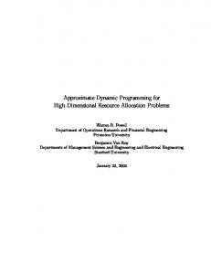
It is assumed that the Mini-Fab operates the 24 hours of the day, 7 days of the week. Each day of operations is composed of two shifts of 12 hours. Also, the metrics utilized to measure the system’s performance include average Work-In-Progress (WIP) inventory, lot completions, and cycle times. A general diagram of the Mini-Fab is depicted in Figure 1. Starts
Buffer 1
Station 1: Diffusion
Buffer 2
Station 2: Ion Impl.
Buffer 3
Station 3: Lithography
Batching
Machines A and B Buffer 5
Machines C and D Buffer 4
Machine E Buffer 6
Batching
Exit Process
Figure 1: General Diagram for the Intel Mini-Fab based on (Kempf 1994) As indicated in Figure 1, the system includes three processing stations: • • •
Station 1 (Diffusion): consists of two tools (Machines A and B) that process batches of three lots of wafers at a given time. Station 2 (Ion Implantation): this station has two tools (Machines C and D) that process the lots of wafers. Station 3 (Lithography): one tool (Machine E) is used in this operation.
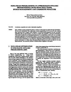
The fabrication of each product considered in the model is completed following the next sequence of six processing steps: Start → Step 1: Diffusion → Step 2: Ion Implantation → Step 3: Lithography → Step 4: Ion Implantation → Step 5: Diffusion → Step 6: Lithography → Exit process. Before starting the processing at each station, the wafer lots are held in six different buffers at the beginning of each step. In addition, in Station 1 there is a batching process that takes place before the batches are placed in Buffers 1 and 5. In our simulation model of the Mini-Fab, we modeled the batching process as it is indicated in Figure 2. As illustrated in the figure, additional entry buffers are utilized, one for each product type, to hold the lots that will be utilized to prepare the batches processed by Station 1. The batching rule depends on the processing step. For instance, in the first processing step the batches can be composed by three lots with any combination of lots of Product A or B, and no more than one lot of Test Wafers. The control problem considered in this research focuses on the decisions of which buffers should be selected to be served next at each station, i.e., job sequencing control. For instance, deciding between serving next Buffer 1 or Buffer 5 in Station 1 when either Machine A or B is available along with the operator PO1. The capacity in the buffers of the system is limited to 18 lots (6 batches) in both Buffer 1 and Buffer 5, and 12 lots in Buffers 2, 3, 4, and 6. In the batching process we assumed a maximum capacity of 18 lots in each of the buffers that hold lots before the batches are prepared. In addition, the model includes a blocking-before-service mechanism, meaning that when a buffer reaches its maximum capacity, the feeding processing step does not start additional lots. The nominal lot starts (i.e., lot releasing rates) are as follows:
1636
Ram´ırez-Hern´andez and Fernandez Entry Buffers (Arrivals or Lots from Station 2)
… New Arrivals … or Lots from Station 2
…
Product A
Product B
Batching
3 Lots/Batch
Buffer 1 or Buffer 5
…
Test Wafers
Batching Process
Figure 2: Modeling of the Batching Process for the Mini-Fab • • •
Product A: 51 lots per week. Product B: 30 lots per week. Test wafers: 3 lots per week.
The processing times for each step in the production flow are given in Table 1. In the experiments we considered both deterministic and exponentially distributed processing times with mean values equal to those indicated in Table 1. Table 1: Production Step Processing Times for the Mini-Fab Model Machines A and B C and D E
Processing Steps 1 and 5 2 and 4 3 and 6
Processing Time Step 1: 225, Step Step 2: 30, Step Step 3: 55, Step
(min) 5: 225 4: 50 6: 10
Before and after the processing at each machine, there are operations of loading and unloading, respectively. In addition, for the processing steps 3 and 6, there are machine setup times depending on changes of the processing step to be performed and type of product to be processed. The operations of loading, unloading, and machine setup are performed by the operators PO1 and PO2 and required specific (deterministic) delays. In addition, other delays such as transportation times for lots and operators between the work stations are also considered. PM operations are included in the model by the specification of PM tasks for each machine in the system. These PM tasks are conducted by the maintenance technician MT1 in each machine during a predetermined (deterministic) amount of time. Moreover, a schedule needs to be provided for such PM operations. The specification of the PM tasks in each machine of the Mini-Fab model are listed in Table 2. Table 2: Duration of Preventive Maintenance Tasks for the Mini-Fab Machines A and B C and D E
Preventive Maintenance Task 75 min every day 120 min every shift 30 min every shift
Similarly, the operators and maintenance technician also follow given schedules that model the breaks and meetings attended by these personnel during the work shifts. In the Mini-Fab model machine failures and emergency repairs are modeled as random events. In particular, only machines C and D can have failures that occur every 50 ± 26 hours (uniformly distributed), and the repair time requires 420 ± 60 minutes to be completed by technician MT1. In the next section we discuss the formulation of the control optimization problem in the Mini-Fab based on the definition of the corresponding state and action spaces as well as the optimization criterion.
1637
Ram´ırez-Hern´andez and Fernandez 3
APPROXIMATE DYNAMIC PROGRAMMING APPROACH
In this section we describe the ADP approach utilized in the optimization of the job sequencing operations for the Mini-Fab model. We first provide details of the formulation of the underlaying Markov Decision Process (MDP) (Puterman 1994) which is utilized later to provide the ADP approach. 3.1 Underlying Markov Decision Process and Optimization Criterion A necessary step before the application of any ADP approaches is the definition of the underlying MDP that models the control problem of interest. In general, and as it is indicated in (Puterman 1994), a MDP is specified by the collection of objects {T, S,U, p(·|s, u), g(s, u)}, where T represents the set of decision epochs (i.e., the times where control actions are made), S is the state space, U is the control space, {p(·|s, u)} are the state transition probabilities, g(s, u) is a cost or reward function, s ∈ S is the state of the system, and u ∈ U is the control. The state is defined using the most representative information of the system which is available to make the appropriate control decisions. In the case of the Mini-Fab model, we defined the state s as follows: s(t) := (B(t), F(t), M(t)), ∀t ∈ T,
(1)
where each component of the state s(t) is described in the following form: •
B(t) represents the buffer levels at time t with B(t) := (b1 (t), b2 (t), b3 (t), b4 (t), b5 (t), b6 (t), bS1,PA (t), bS1,PB (t), bS1,TW (t), bS5,PA (t), bS5,PB (t), bS5,TW (t)),
•
where {b1 , ..., b6 } represent the levels of Buffers 1 to 6, and {bS1,PA , bS1,PB , bS1,TW , bS5,PA , bS5,PB , bS5,TW } are the levels of the buffers (one for each product type) included in the batching processes for the processing steps 1 and 5 (see Figure 2), respectively. In addition, PA, PB, and TW stands for Product A, B, and Test Wafers, respectively, and S1, S5 stands for the processing steps 1 and 5, respectively. F(t) provide the indication of failures in Machines C and D, and it is defined as follows: F(t) := ( fC (t), fD (t)),
•
(2)
(3)
where fC , fD are indicators of failures in Machines C and D, respectively, with fC , fD ∈ {0, 1}. For instance, fC (t) = 1 and fD (t) = 0 indicates that at time t Machine C is in failure while Machine D is not. We assumed that when a machine enters in a failure state it remains in that state until the emergency repair is completed and the machine is put back in service. M(t) indicates the occurrence of PM operations in the machines: M(t) := (mA (t), mB (t), mC (t), mD (t), mE (t)),
(4)
where mA , ..., mE indicate if a PM task is underway at time t in Machines A to E, respectively, with fA , ..., fE ∈ {0, 1}. For instance, mA (t) = 1 and mB (t) = 0 indicates that at time t Machine A is receiving a PM operation while Machine B is not. The state space is finite given that the buffers have finite capacity. The dimension of such space can be computed knowing that there are 8 buffers of 18 lots of capacity, 4 buffers of 12 lots of capacity, and 7 state components with binary values. Thus, the dimension of the state spaces is as follows: |S| = 188 × 124 × 27 ≈ 2.9249 × 10¹⁶ different states. The decision epochs are assumed to be the times in which any change in the state occurs. That is, the times for any lot arrival, departure, failure and preventive maintenance occurrences, as well as the times for completions of any maintenance task (including emergency repairs). The control u is defined as follows: u(s) := (u1 (s), u2 (s), u3 (s), u4 (s), u5 (s), u6 (s)), ∀ s ∈ S,
1638
(5)
Ram´ırez-Hern´andez and Fernandez where u1 , ..., u6 ∈ {0, 1}, with ui = 1 representing the action of selecting a lot (or batch) from Buffer i, with i = 1, ..., 6, to be serve next in the corresponding work station. Similarly, ui = 0 represents the action of no selecting Buffer i for service. From Figure 1 notice that there are three pairs of buffers that compete for service in the Mini-Fab. Buffers 1 and 5 compete for service in station 1, Buffers 2 and 4 in station 2, and Buffers 3 and 6 in station 3. Moreover, we assume that there is a set of constraints, U (s), for these control actions and such that u(s) ∈ U (s) ∀s ∈ S. One of the constraints defined for U (s) is based on the fact that at each decision epoch t ∈ T only one lot (or batch) from each pair of competing buffers is selected at the time to receive service. These constraints are defined as follows: u1 = 1 − u5 , u2 = 1 − u4 , and u3 = 1 − u6 . We also assumed that a non-idling policy is applied to avoid work starvation in the machines. Thus, if one of the buffers competing for service is empty while the other has at least one job, then the non-empty buffer receives immediate priority for service. Another constraint is that related to the blocking-before-service mechanism. In this case any control ui = 0 if the i + 1-th buffer reaches its maximum capacity such that overflow is avoided, with i = 1, ..., 5. Because of the complexity of the Mini-Fab model, the transition probabilities {p(·|s, u)} cannot be explicitly specified. However, for the purpose of applying a simulation-based ADP approach it will be sufficient to know that given some decision rule or control policy, then state transitions in the system will follow some probabilistic distribution, and that the system have the Markov Property (Sutton and Barto 1998) which is essential for the application of ADP. Thus, a simulation model is utilized instead to generate the necessary information of state-transition dynamics that will be later utilized in the optimization of the control actions. Moreover, as it will be discussed later, we exploit certain structural properties of the optimal control within the ADP algorithm. The last object to be defined in the MDP formulation corresponds to the cost or reward function g(s, u). Before defining such object, we first assume that the average WIP inventory will be the metric to be utilized to measure the performance of the Mini-Fab under a given control policy. In addition, we assume that the Mini-Fab operates in a continuous form such that there are neither final nor absorbing states, and that the decision epochs are discrete times corresponding to the times where the state of the system changes. Thus, we define the following infinite horizon average cost criterion as the performance index to be utilized in the optimization problem: 1 J (s) = lim E N→ N
�
N−1
�
g(sk ) |s0 = s
,
(6)
k=0
where J (s) is the average cost function under policy ∈ ad , where ad is the set of admissible control policies, g(s) is the one-stage cost function, s0 is the initial state, with s ∈ S, and k is the state transition index. For simplicity we assume that there are no costs associated with the control actions. Then, the one-stage cost function g(s) is a function of the state only. Notice that a policy ∗ ∈ ad such that J ∗ (s) = min ∈ad J (s) ∀ s ∈ S is said to be an optimal average cost policy. Given the previous optimization criterion, we construct the one-stage cost function g(s) with those elements of s that will affect the WIP levels in the system and such that J reflects a direct measure of the long-run average WIP in the Mini-Fab. Thus, we proposed the following one-stage cost function: → − → − → − g(s) := B · cTB + F · cTF + M · cTM ,
(7)
→ − → − → − where B , F , and M are vectors containing the elements specified for B(t), F(t), and M(t) given in (2)-(4), respectively, and → − cB ∈ R12 , cF ∈ R2 , and cM ∈ R5 are vectors of nonnegative cost coefficients. The term B · cTB provides a measure of total → − → − amount of jobs waiting for service in the system. The remaining terms F · cTF and M · cTM are included to provide additional costs derived from failures and maintenance operations. Such terms are included considering that failures and PM tasks directly decrease the capacity of service in the stations which in turn increases the resulting WIP levels in the Mini-Fab. Under specific conditions for the corresponding MDP, e.g., see (Puterman 1994, Meyn 2008), it is possible to formulate the following Average-Cost Optimality Equation (ACOE) (Puterman 1994): �
�
∗ + h∗ (s) = min
u∈U (s)
g(s) + p(s� |s, u)h∗ (s) , ∀ s ∈ S,
(8)
s�
where ∗ is a scalar that corresponds to the optimal average cost and such that ∗ = min ∈ad J (s) ∀s ∈ S, s� ∈ S is the next state, and h∗ (s) is the relative or differential-cost function (Bertsekas 2000). Also, a stationary policy that provide control actions that minimize the right-hand side of (8) is said to be an optimal average cost policy.
1639
Ram´ırez-Hern´andez and Fernandez Results reported in (Meyn 2008, Theorem 4.1.3, pp.108, Theorem 9.0.3, pp.377) indicate that an optimal solution for the ACOE exists for scheduling problems in queueing networks under conditions that include that the one-stage cost function g(s) can be extended to defined a norm on Rl , where l is the number of components of the state s, and that there exist a stabilizing control policy (Meyn 2008) for the system. Such conditions hold for the control optimization problem of the Mini-Fab model. That is, the one-stage cost function g(s) given in (7) is linear in the state; therefore, it is a norm on is a norm on R19 . Also, as it is reported in (Meyn 1997), it is known that certain dispatching rules, e.g., the Last-Buffer-First-Served rule, provide stabilizing policies for general RLM models. Thus, the optimization problem that will be addressed via simulation-based ADP is to find a policy ADP ∈ ad such that ADP ≈ ∗ , where ADP represents the average cost under the policy generated via simulation-based ADP. The details of the ADP approach utilized in such optimization problem are presented next. 3.2 A Simulation-Based ADP Approach for Average-Cost Problems Based on an Actor-Critic Architecture The ADP approach applied in this control optimization problem utilizes the same Actor-Critic architecture reported in (Ram´ırez-Hern´andez and Fernandez 2007b) for the control of simple reentrant line manufacturing models. Such architecture is depicted in Figure 3. As shown in the figure, the simulation model of the Mini-Fab is utilized to generate both traces of the state s and the one-stage cost values g(s). Such measures are utilized by an ADP agent to tune a vector of parameters r for a linear approximation structure utilized to estimate the optimal differential cost hˆ ∗ (s, r) ≈ h∗ (s). Such process of estimating the optimal differential cost is indicated as the critic in the architecture. The estimations hˆ ∗ (s, r) are then utilized to generate approximations to the optimal control uˆ∗ ≈ u∗ by the actor or controller. g (s) uˆ *
Mini-Fab (Simulation Model)
ADP Agent
s
r Controller (Actor)
hˆ * ( s, r )
Parametric Estimation of the Optimal Differential Cost (Critic)
Figure 3: An actor-critic architecture for ADP (adapted from Ram´ırez-Hern´andez and Fernandez 2007b) The ADP agent in this Actor-Critic architecture utilizes the average cost temporal-difference learning TD( ) algorithm reported by (Tsitsiklis and Van Roy 1999) and a gradient descent approach to tune the vector of parameters r. Moreover, as in (Tsitsiklis and Van Roy 1999) the approximation structure hˆ ∗ (s, r) utilized is assumed to be linear in the parameters r and is defined as follows: − (s) · rT ≈ h∗ (s), ∀s ∈ S, hˆ ∗ (s, r) := →
(9)
− (s) is a vector of basis functions (Bertsekas and Tsitsiklis 1996, Sutton and Barto 1998). where → As indicated in (Tsitsiklis and Van Roy 1999), the TD( ) algorithm uses the following temporal-differences as the error to guide the tuning of the parameters with a gradient descent method: ˆ k+1 , rk ) − h(s ˆ k , rk ), dk = g(sk ) − k + h(s
(10)
where k represents an approximation of the optimal average cost ∗ at the k-th state transition. Such estimate is updated as follows:
k+1 = (1 − k (sk , uk )) · k + k (sk , uk ) · g(sk ),
(11)
with 0 defined as an initial estimation of ∗ and k (sk , uk ) as a scalar step size which decreases with the number of visits to the state-control pair (sk , uk ). Thus, the parameters rk are updated with the following iterative equation: rk+1 = rk + k (sk , uk ) · dk · zk ,
1640
(12)
Ram´ırez-Hern´andez and Fernandez p
where k (sk , uk ) := v (s ,u ) is another step size in the algorithm and for which p ∈ R+ is a small scalar, vk (sk , uk ) represents the k k k number of visits to the state-control pair (sk , uk ), with , with v0 (s0 , u0 ) ≥ 1. Also, it is assumed that k (sk , uk ) = c · k (sk , uk ) ∀ k, with c ∈ R+ , and zk is the vector of elegibility traces (Bertsekas and Tsitsiklis 1996, Sutton and Barto 1998) which is updated as follows: − (sk+1 ), zk+1 = · zk + →
(13)
where z−1 is initialized as a zero vector and ∈ [0, 1) is the parameter for the TD( ) algorithm. In addition, it is assumed that the step size k (sk , uk ) is such that follows the usual assumptions for stochastic iterative algorithms (Bertsekas and Tsitsiklis 1996) 2 under which k=0 k (sk , uk ) = and k=0 k (sk , uk ) < . The flow of the TD( ) algorithm utilized described here follows closely that one indicated in (Ram´ırez-Hern´andez and Fernandez 2007b) for a discounted cost criterion. To complete the description of the ADP approach, we now focus on the definition of the actor or controller. For this task we exploit structural properties of the optimal control problem which are derived from the optimality equation. As reported in (Ram´ırez-Hern´andez and Fernandez 2007b, 2009), for optimal job sequencing problems in RLM models, the optimal control decisions are determined by the expected savings in costs derived from applying a given control action. Such structural property is also observed in the ACOE given in (8). Thus, based on the ACOE and the structural properties of the optimal control problem, the following is the actor or controller for the ADP algorithm that approximates the optimal control actions: � � �1 (s, r) + u2 · �2 (s, r) + · · · + u6 · �6 (s, r) , ∀ s ∈ S, (14) u1 · uˆ∗ (s) = arg max u(s)∈U (s)
�n (s, r) is an approximation of the expected savings in optimal differential costs with where � � �n (s, r) := n · hˆ ∗ (s, r) − hˆ ∗ (Bn s, r) ,
(15)
where n represents the expected time required for the state transition from s to Bn s as a result of taking the control action un = 1 (i.e., service rate of jobs from buffer n), Bn s is a mapping from S to S that determines the next state departing from s with n = 1, ..., 6, and hˆ ∗ (s, r) is the approximation of the optimal differential cost h∗ (s) given the vector of parameters r tuned via a TD( ) algorithm. As noticed from (14), the actor aims to provide control actions that maximize the total amount of average savings in the optimal differential costs. As such these control actions aim to minimize of the right-hand side of the ACOE given in (8). In the ADP algorithm described above we also incorporated the possibility of exploration of the control space by using an -greedy policy approach (Sutton and Barto 1998, Bertsekas and Tsitsiklis 1996). Thus, exploration on the control space is performed by selecting a random control action with a small probability (uniformly distributed). In the next section we present results from simulation experiments on which both dispatching rules reported in the literature and control policies generated via ADP were utilized in the control of the Mini-Fab model. 4
SIMULATION EXPERIMENTS
In order to evaluate the performance of the policies obtained with the proposed simulation-based ADP approach, several simulation experiments were conducted under different operational conditions in the Mini-Fab model. Because there are no known optimal solutions for the optimization control problem of the Mini-Fab described in section 3, then we utilized several dispatching rules that have been utilized in other RLM models and that have been reported in the literature in e.g., (Wein 1988, Kumar 1993, Kumar and Kumar 2001). The following is the initial list of dispatching rules that were tested with the Mini-Fab model: • • •
First-In-First-Out (FIFO): this is a well known rule that gives service to the jobs or lots in their order of arrival, giving the highest priority to the earliest arrival. This rule is also known as the First-Come-First-Served (FCFS) rule. First-Buffer-First-Served (FBFS): is a dispatching rule that gives priority of service to the job that is at the earliest stage of the production process. Last-Buffer-First-Served (LBFS): this rule represents the complete opposite of the FBFS rule and gives priority of service to jobs that are at the latest stage of the production process. This rule has been designed to reduce the
1641
Ram´ırez-Hern´andez and Fernandez
• • •
cycle-time in the system and is also equivalent to the so-called Shortest Remaining Processing Time (SRPT) rule and to the Least Slack policy with parameters = 0 (Kumar 1993). Shortest Processing Time (SPT): the priority of service with this rule is given to the jobs that have the shortest processing time at the corresponding work station. Longest Processing Time (LPT): this rule is the opposite of the SPT rule by giving priority of service to the jobs with the longest processing time at the corresponding work station. Least-Work-Next-Queue (LWNQ): this rule follows an heuristic approach for regulating the inventory levels of each work station. As such, this rule gives priority of service to the jobs that after completion of service will join the queue with the smallest inventory.
From the previous list, and after evaluating each dispatching rule for the control of the Mini-Fab model and for each of the experiments described later in this section, the rules LBFS and LWQN were selected for a final comparison against control policies obtained via ADP. The remaining dispatching rules in the list above provided a deficient performance when compared against policies generated by ADP and against the LBFS and LWNQ rules. Thus, in this section we only present the results from simulation experiments with these two dispatching rules and the best policies generated via ADP. As it will be discussed later in this section, both the dispatching rules and the policies generated via ADP obtained similar performances. However, it is expected that the policies obtained via ADP can be improved by further refining of the approximation structure employed as well as that ADP may offer additional advantages over static rules, e.g., control policies that can be adapted to operational changes in the fab and designed to reduce specific performance metrics. Four different simulation experiments were performed under two different and arbitrary PM schedules, and under either deterministic or random processing times in the machines. Such random times were assumed to be exponentially distributed with means equal to the processing times indicated in Table 1. Table 3 lists the type of experiments conducted, and Table 4 provide details of the two daily PM schedules utilized in the experiments where the start times for the PM tasks are given in the usual time format hours:min:secs and assuming that the first work shift starts at 00:00:00. Table 3: Simulation Experiments Conducted to Evaluate the Performance of Different Control Policies in the Mini-Fab Model Experiment # 1 2 3 4
PM Schedule Schedule 1 Schedule 1 Schedule 2 Schedule 2
Processing Times Deterministic Random (exp. dist.) Deterministic Random (exp. dist.)
Table 4: PM Schedules 1 and 2 for the Mini-Fab Model Machine A B C D E
PM Task Start Time Schedule 1 Schedule 2 06:00:00 06:00:00 12:00:00 08:00:00 00:00:00 06:00:00 08:00:00 04:00:00 03:00:00 03:00:00
The following is a list of general conditions considered in the generation of control policies with the proposed ADP approach: • • •
Both the Mini-Fab simulation model and the ADP approach were implemented with the simulation software AutoMod (Applied Materials 2009). The generation of control policies with ADP was performed with a “learning process” that consisted of 400 simulation replications of 10000 hours each. Such number of replications and simulation length was sufficient to obtain proper convergence of the parameters in r The approximation structure hˆ ∗ (s, r) utilized was composed of 19 basis functions. The first 18 basis functions corresponded to each of the components of the state s specified in (2)-(4), excluding the indicator mE . Experimentally it was determined that the addition of the later indicator did not improved the performance of policies being generated
1642
Ram´ırez-Hern´andez and Fernandez
•
•
via ADP. Therefore, such indicator was not included as a basis function in the final approximation structure hˆ ∗ (s, r). A possible reason for this behavior could be the fact that the PM task in Machine E is the one with the smallest duration, so it probably did not impact significantly the selection of control actions. The remaining basis function selected was a constant with value equal to 1. Thus, the vector of parameters r has 19 components and r ∈ R19 . In addition, the components of the vectors cB , cF , and cM , were set to 1, except for the last component in cM that wast set to zero given that the state component mE was not considered in the approximation structure. Experimentally, it was determined that the best policies generated via ADP were obtained with initial values of 0 ∈ {47, 48, 49, 50, 51, 52, 53}, p ∈ {0.0001, 0.001, 0.002}, and ∈ {0.7, 0.9, 0.95}. In addition, we set k (sk , uk ) = k (sk , uk ) and during the approximation process the the value of p was decreased at different simulation replications to refine the quality of the control policies obtained. An -greedy policy approach was utilized with values of ∈ {0, 0.0001, 0.00001}. In general, is was observed that a small amount of exploration w.p. = 0.0001 was beneficial in the refinement of the policies generated via ADP.
The evaluation of the control policies obtained with ADP as well as the rules LBFS and LWQN was conducted via multiple simulation replications on which the statistics of the average WIP and average cycle time were collected. Between 50 to 100 replications of 3650 days each were ran for each evaluation and the statistics were computed considering a warm-up period of 365 days. The results of the experiments are provided in Tables 5 - 8 where the statistics of average Work-In-Process (WIP), given in lots, and average Cycle-Time (CT), given in hours, are listed with the corresponding 95% confidence intervals for each of the product types produced by the Mini-Fab. We included the average CT in the results because it is an important performance index commonly utilized in semiconductor manufacturing systems, and because by Little’s law (Little 1961) it is known that low average WIP levels will lead to short average CT. Therefore, with the goal of reducing the average WIP levels in the system we are also aiming to reduce the average CT. As mentioned earlier, the performance for the control policies FIFO, FBFS, SPT, and LPT were not included because these presented a poor performance. For instance, the SPT rule provided an average WIP for product A of 41.06 lots and an average cycle time for product B of nearly 500 hours. Table 5: Performance of Control Policies in the Mini-Fab Model for Experiment #1 Control Policy LBFS ADP LWNQ
Product A
Product B
Test Wafers CT
WIP
CT
WIP
CT
WIP
[30.71, 30.79] [31.04, 31.13] [32.36, 32.46]
[370.91, 374.96] [376.78, 381.22] [385.11, 390.09]
[18.16, 18.21] [18.35, 18.41] [19.10, 19.16]
[375.46, 379.59] [381.31, 381.22] [389.30, 394.28]
[1.96, 1.99] [1.99, 2.02] [2.06, 2.09]
[363.20, 367.63] [369.61, 374.32] [378.36, 383.86]
Experiment #1: PM Schedule 1 and Deterministic Processing Times.
Table 6: Performance of Control Policies in the Mini-Fab Model for Experiment #2 Control Policy LBFS ADP LWNQ
Product A
Product B
Test Wafers CT
WIP
CT
WIP
CT
WIP
[30.78, 30.86] [31.54, 31.61] [32.30, 32.38]
[375.45, 379.99] [385.33, 388.54] [389.68, 394.54]
[18.17, 18.23] [18.60, 18.64] [19.02, 19.09]
[379.47, 384.00] [389.53, 392.80] [393.91, 398.95]
[1.94, 1.97] [2.01, 2.03] [2.07, 2.09]
[367.94, 372.71] [378.93, 382.48] [381.56, 386.86]
Experiment #2: PM Schedule 1 and Random Processing Times (Exp. Dist.).
Table 7: Performance of Control Policies in the Mini-Fab Model for Experiment #3 Control Policy LBFS ADP LWNQ
Product A
Product B
Test Wafers CT
WIP
CT
WIP
CT
WIP
[30.25, 30.32] [30.63, 30.69] [31.79, 31.87]
[332.56, 337.02] [337.33, 339.82] [340.09, 344.13]
[17.85, 17.90] [18.11, 18.14] [18.81, 18.85]
[336.58, 341.09] [341.51, 343.99] [344.13, 348.19]
[1.93, 1.95] [1.97, 1.99] [2.04, 2.06]
[326.06, 330.32] [330.96, 333.96] [334.22, 338.57]
Experiment #3: PM Schedule 2 and Deterministic Processing Times.
The results indicated in Tables 5 to 8 show that in general the control policy that yielded the minimum average WIP levels in the Mini-Fab was the LBFS rule. However, the performance of the policies obtained via ADP followed closely
1643
Ram´ırez-Hern´andez and Fernandez Table 8: Performance of Control Policies in the Mini-Fab Model for Experiment #4 Control Policy LBFS ADP LWNQ
Product A
Product B
Test Wafers CT
WIP
CT
WIP
CT
WIP
[30.35, 30.43] [30.75, 30.80] [31.83, 31.90]
[339.62, 343.98] [343.48, 346.03] [347.90, 351.62]
[17.93, 17.98] [18.16, 18.20] [18.76, 18.82]
[343.64, 348.00] [347.55, 350.17] [351.43, 355.28]
[1.94, 1.96] [1.97, 1.98] [2.02, 2.05]
[333.37, 338.07] [337.40, 340.34] [341.59, 346.04]
Experiment #4: PM Schedule 2 and Random Processing Times (Exp. Dist.).
with maximum difference in performance with respect to the LBFS rule of approximate 3.6%. The LBFS rule also provided the best minimization in the average cycle time in most of the experiments except in Experiment #4, where the policy generated via ADP obtained a statistical match for cycle time performance obtained by such rule (see Table 8). Also, in all the experiments conducted the policies generated by ADP performed better than the LWQN rule in terms of both average WIP and average cycle time. Only in Experiment #2 there was a statistical match in the average CT between these policies. The results presented here validated the applicability of the proposed simulation-based ADP approach for the optimization of the job sequencing operations in the Mini-Fab. These results also served as a proof of concept for the application of ADP in more complex RLM models than those that had been considered in our previous research (Ram´ırez-Hern´andez and Fernandez 2007a, 2007b). Moreover, the results validated the utilization of the structural properties of the optimal control problem in the formulation of the actor or controller within the Actor-Critic architecture which is defined by estimations of the savings in optimal differential costs derived from taking particular actions in the system (e.g., see (15) and (14)). 5
CONCLUSIONS
We presented initial results on the application of a simulation-based ADP approach for the control of the benchmark model of a semiconductor fab denominated the Mini-Fab. Results from this research validated the applicability of such ADP approach in the control of the Mini-Fab model by showing good performances when compared against the performance of several dispatching rules commonly utilized in semiconductor fabs. The results also suggest that the advantage in these particular experiments is on the side of the dispatching rules LBFS and LWNQ because these are simpler to implement than ADP and provide similar performance. However, it is important to notice that in these initial experiments we only utilized a simple approximation structure, and as reported in (Ram´ırez-Hern´andez and Fernandez 2007a), other structures may significantly improve the performance of the policies being generated via ADP. As such, additional research is required to refine the approximation structure and possibly improve the performance yielded by policies generated via ADP. Simulation-based ADP also offers the advantage of generating control policies that are adapted to the operational conditions being assumed in the system’s simulation model and according to the optimization criterion selected. Thus, policies generated via ADP may have the advantage over other static policies by which their performance is affected by operational variations in the system or that have been designed or conceived to improve only specific metrics. Another advantage that ADP could offer with respect to other control strategies is the possibility of integrating other fab optimization problems within a more globalized optimization of the fab. REFERENCES Bertsekas, D. P. 2000. Dynamic programming and optimal control. Second ed, Volume II. Bellmont, MA: Athena Scientific. Bertsekas, D. P., and J. N. Tsitsiklis. 1996. Neuro-dynamic programming. Bellmont, MA: Athena Scientific. Kempf, K. 1994. Intel five-machine six step mini-fab description. Available via [accessed March 29, 2009]. Kumar, P. R. 1993. Re-entrant lines. Queueing Systems: Theory and Applications 13:87–110. Kumar, P. R. 1994. Scheduling semiconductor manufacturing plants. IEEE Control Systems Magazine 39 (11): 33–40. Kumar, S., and P. R. Kumar. 2001. Queueing network models in the design and analysis of semiconductor wafer fabs. IEEE Transactions on Robotics and Automation 17 (5): 548–561. Little, J. D. C. 1961. A proof for the queueing formula: L= w. Operations Research 9 (3): 383–387. Meyn, S. 2008. Control techniques for complex networks. New York, NY: Cambridge University Press. Meyn, S. P. 1997. The policy iteration algorithm for average reward markov decision processes with general state space. IEEE Transactions on Automatic Control 42 (12): 1663–1680.
1644
Ram´ırez-Hern´andez and Fernandez Powell, W. B. 2007. Approximate dynamic programming: Solving the curses of dimensionality. Hoboken, NJ: WileyInterscience. Puterman, M. L. 1994. Markov decision processes: Discrete stochastic dynamic programming. New York, NY: John Wiley & Sons, Inc. Ram´ırez-Hern´andez, J. A., and E. Fernandez. 2005, December 12-15. A case study in scheduling reentrant manufacturing lines: Optimal and simulation-based approaches. In Proceedings of the 44th IEEE Conference on Decision and Control, and the European Control Conference 2005, 2158–2163. Seville, Spain. Ram´ırez-Hern´andez, J. A., and E. Fernandez. 2007a, April. An approximate dynamic programming approach for job releasing and sequencing in a reentrant manufacturing line. In Proceedings of the 2007 IEEE Symposium on Approximate Dynamic Programming and Reinforcement Learning (ADPRL 2007), 201–208. Honolulu, HI. Ram´ırez-Hern´andez, J. A., and E. Fernandez. 2007b, December 13-15. Control of a re-entrant line manufacturing model with a reinforcement learning approach. In Proceedings of the Sixth International Conference on Machine Learning and Applications (ICMLA’07), 330–335. Cincinnati, OH. Ram´ırez-Hern´andez, J. A., and E. Fernandez. 2009. Simulation-based approximate dynamic programming for near-optimal control of re-entrant line manufacturing models. submitted to IEEE Transactions on Automation Science & Engineering. Ram´ırez-Hern´andez, J. A., H. Li, E. Fernandez, C. R. McLean, and S. Leong. 2005, December. A framework for standard modular simulation in semiconductor wafer fabrication systems. In Proceedings of the 2005 Winter Simulation Conference, ed. M. E. Kuhl, N. M. Steiger, F. B. Armstrong, and J. A. Joines, 2162–2171. Piscataway, New Jersey: Institute of Electrical and Electronics Engineers, Inc. Shen, Y., and R. Leachman. 2003. Stochastic wafer fabrication scheduling. IEEE Trans. on Semic. Manufac. 16 (1): 2–14. Si, J., A. G. Barto, W. B. Powell, and D. W. II. (Eds.) 2004. Handbook of learning and approximate dynamic programming. IEEE Press, Wiley-Interscience. Sutton, R. S., and A. G. Barto. 1998. Reinforcement learning: An introduction. Cambridge, MA: MIT Press. Applied Materials 2009. AutoMod. Available via [accessed March 31, 2009]. Modeling and Analysis For Semiconductor Manufacturing Laboratory (MASMLab), Arizona State University 2003. Test bed. Available via [accessed March 29, 2009]. Tsakalis, K. S., J. J. F. Godoy, and A. A. Rodriguez. 1997. Hierarchical modeling and control for re-entrant semiconductor fabrication lines: A mini-fab bechmark. In Proceedings of the 6th IEEE International Conference ETFA, 514–519. Tsitsiklis, J. N., and B. Van Roy. 1999. Average cost temporal-difference learning. Automatica 35:1799–1808. Uzsoy, R., C. Lee, and L. A. Martin-Vega. 1994. A review of production planning and scheduling models in the semiconductor industry part II: Shop-floor control. IIE Transactions 26 (6): 44–55. Wein, L. M. 1988. Scheduling semiconductor wafer fabrication. IEEE Trans. on Semiconductor Manufacturing 1:115–130. AUTHOR BIOGRAPHIES ´ ´ ANDEZ received the B.Sc., ”Licenciatura,” and M.Sc. degrees in Electrical Engineering from JOSE´ A. RAMIREZ-HERN The University of Costa Rica in 1995, 1996, and 1999 respectively. Currently, he is a Ph.D. candidate at the Department of Electrical & Computer Engineering at the University of Cincinnati. His research interests include Markov decision processes, dynamic programming, and simulation-based optimization methods. He is member of IEEE and INFORMS. His e-mail address for these proceedings is . EMMANUEL FERNANDEZ received a Ph.D. degree in Electrical and Computer Engineering from The University of Texas at Austin in 1991. He has M.Sc. degrees from the University of Oklahoma, Norman, in Applied Mathematics (1986) and Electrical Engineering (1985), and a B.Sc. in Electrical Engineering from the University of Costa Rica (1983). From 1991 to 2000 he was with the Systems & Industrial Engineering Department at the University of Arizona, Tucson. Since 2000, he is with the Electrical & Computer Engineering Department at the University of Cincinnati, where he is an Associate Professor and Director of the “Laboratory for Systems Modeling & Information Technology” (URL: ). His research areas of expertise are stochastic models, stochastic decision and control processes, and mathematical and computational operations research. His interests in applications are broad, spanning across the areas of manufacturing, operations and management, telecommunication, logistics, algorithms and software/Internet tools. He is a member of INFORMS, SIAM, and Senior member of IEEE and IIE. His e-mail address for these proceedings is .
1645