A simulation-based learning environment assisting scientific activities based on the classification of 'surprisingness' Tomoya Horiguchi Faculty of Maritime Sciences, Kobe University, Japan
[email protected] Tsukasa Hirashima Deptartment of Information Engineering, Hiroshima University
[email protected] Abstract: In this paper, we propose a general framework of the learning environment in which the system can explicitly assist a learner’s scientific activity. A learner can improve her hypothesis and model of the domain developmentally with the guidance of the tutoring system. First, we present the framework for generally representing the models of the domain and their relations. Then, we classify the differences between the erroneous and correct models’ behaviors of physical systems. This classification is conducted by a process ontology of physical systems, and used as the guideline for representing the knowledge of model modifications. The example of how our method works in an elementary mechanics problem is also presented.
Introduction The ‘microworld’ provides a learner virtual experiences about physical phenomena in computer-simulated environment. It has been regarded as a promising method for assisting the ‘constructivistic’ learning (learner-driven discovery and acquisition of knowledge) since the early stage of the CAI research. However, it has also been pointed out that providing a simulator is insufficient, because a computer-simulation supports only a small part of a scientific activity, which involves (1)hypothesis formation, (2)planning and performing an experiment, (3)hypothesis evaluation through the result. Therefore, in order to assist the high-level scientific activities such as hypothesis formation and evaluation, a lot of researches have been made by technological, psychological and pedagogical approaches (Wenger 90). In artificial intelligence approach, the techniques have been developed to make tutoring systems understand and explain the contents of scientific reasoning themselves by modeling the domain knowledge explicitly. Especially, qualitative reasoning provides a technique to simulate not only the physical phenomena but also the conceptual knowledge of the domain. This makes it possible for a learner to explore the world of the conceptual models. With referring the presented knowledge by tutoring systems, she could (re)construct her knowledge of the domain. On the other hand, in scientific activity, the most important trigger for learning is to recognize an error and to modify the knowledge concerned with it. Assume a learner observes a phenomenon which she can’t explain by her hypothesis or model. The reconstruction of knowledge occurs (only) when she understands the meaning of the difference between her prediction and the result, and modifies her hypothesis or model correctly (Perkinson 84). From this viewpoint, the achievements of artificial intelligence approach are not sufficient. Whether it is of physical phenomena or of conceptual knowledge, the knowledge reasoned and presented by tutoring systems is the ‘correct’ knowledge. When a learner has ‘erroneous’ knowledge, it is up to her to find out how to reconstruct her knowledge (with referring to the correct one). If one make tutoring systems assist such a task directly, a lot of knowledge for it must be represented depending on the individual domain and situation. For example, White and her colleague developed the systems which help a learner improve her mental model ‘developmentally’ (White 90, 93). In the learning environments, she learns in a series of microworlds step by step. Since the knowledge necessary for solving problems in the microworlds gets complicated gradually, she can improve her hypothesis or model developmentally. However, even in this case, the knowledge presented by the systems is the correct one. What helps a learner reconstruct her knowledge is not the microworlds themselves but their unitization and serialization. Such a ‘curriculum’ must be designed by human tutors based on the detailed
domain analysis. The systems don’t have the ability to reason about a learner’s error (that is, the ability to identify its cause and how to correct it). Of course, it is difficult to reuse the knowledge and mechanism of these systems. In this paper, we propose a general framework of the learning environment in which the system can explicitly assist a learner’s scientific activity (especially the recognition and correction of errors in her hypothesis or model) in microworld. First, we present the framework for generally representing the models of the domain and their relations. Then, we classify the differences between the erroneous and correct models’ behaviors of physical systems. This classification is conducted by a process ontology of physical systems, and used as the guideline for representing the knowledge of model modifications.
The System Design In our research, we define the scientific activity as follows: First, a learner forms the initial model to explain the behavior of the physical system based on her experiences and knowledge (or some assumptions). Then, she plans an experiment and performs it. If there is some difference between her prediction and the result, she evaluates its meaning and modifies her model. This procedure is continued until she gets the ‘correct’ model. In order for the success of such learning in microworld, one of the key points is to understand the meaning of the difference between the observation (result of the experiment) and prediction by the model, and to modify the model appropriately. The modification of the model, which involves both the adjustment of parameters and the change of the fundamental assumptions, is often the difficult task for a learner. Therefore, some assistance for it is necessary. In this paper, we propose a computational framework for explicitly assisting the model development, which hasn’t been discussed in a general framework because of its domain dependency. Definition and Requisites Model We define a model of the physical system as a set of parameters (state variables and constants) and constraints between them. The parameters and their domains/values are determined depending on what kinds of physical objects and physical processes are considered in the model, that is, modeling assumptions. A model may consist of some submodels which are bound with boundary conditions. The task of a learner is to construct the model of the physical system based on some assumptions, and to make it the same as the ‘correct’ model (set by a tutor) through experiments and modifications. Domain knowledge In order to make such a learning environment, we use the ‘graphs of models’ (Addanki 89, 91) as the basic framework. A graph of models is a graph which describes a set of the possible models of the physical system and the conditions for changing the models. Each node stands for a possible model, and each edge stands for a possible transition between two models (by changing the assumption(s)). To each edge, the condition for going from one model to the other is attached. Each model corresponds to each (possible) combination of the assumptions in the domain. In this framework, when some conflicts occur in one (inappropriate) model, the candidates of model transition to eliminate the conflicts are inferred. The conflicts can occur in two ways: empirically or internally. An empirical conflict occurs when there are some differences between the values derived from a model (predicted values) and the ones measured in the world (observed values). Internal conflicts occur when some observed values are inconsistent with one of the modeling assumptions. The outline of the inference is as follows: (step-1) from the conflict between the predicted and observed values, the ‘delta-vectors’ are generated, each of which indicates the parameter to be modified and its direction (to be increased/decreased). The list of delta-vectors is called ‘delta-list.’ (step-2) by using the ‘parameter-change-rules’ (which describes the qualitative effect of assumption change on parameter values), the candidates of model transition (from the current model to its neighbors) are determined which satisfy the delta-list the most.
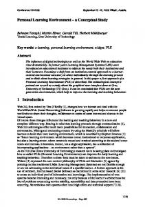
thrown with the initial velocity v0
swept with ‘broom’ uniformly
M1
M2
mu2
mu1
x0 = 0 v0
x1 v1
Tice
x2 v2
Figure 1a. the ‘Curling-like’ situation Graph-A Graph-B Model-1 - with no friction v = v0
Model-2 - with friction
Model-4 - elastic collision Model-3 - with friction - the heat generated v = !(v0 2- 2"1M1gx) 2 v’ = !(v1 - 2"2M1g(x-x 1)) Tice > 0
v1’ = (M1- M2)vB/(M1 +M2), v2’ = 2M1vB/(M1 +M2)
Model-5 - inelastic collision v1’ = (M1- eM2)vB/(M1 +M2), v2’ = (1+ e)M1vB/(M1 +M2) (0 < e < 1)
2
v = !(v0 - 2"1M1gx) Tice = 0
Boundary condition: vB = v2
Figure 1b. the Graphs of models (Example-1) Figure 1a shows a ‘curling-like’ situation. Suppose a player makes a ‘stone’ slide on the ice to let it collide with another stone. At the position x0, stone M1 is thrown with the initial velocity v0, then slides on the ice rightward until it collides with stone M2 at the position x2. The ice between the position x1 and x2 (described as ‘the interval x1-x2’) is swept with ‘broom’ uniformly before stone M1 reaches the position x1. When modeling the behavior of this physical system, the graph of models shown in Figure 1b is obtained according to what physical processes are considered. Graph-A corresponds to the sliding motion of M1 in the interval x0-x2 and Graph-B corresponds to the collision at the position x2. Both graphs are combined by the boundary condition. Each model in these graphs is based on the following modeling assumptions: Model-1: M1 moves uniformly because no force works on it. Model-2: M1 moves with deceleration because of the frictional force from the ice. Sweeping the interval x1-x2 has no influence. Model-3: M1 moves with deceleration because of the frictional force from the ice. In this model, sweeping makes the surface of ice melt, so the frictional force in the interval x1-x2 is smaller than the one in the interval x0-x1. In addition, the temperature of the surface of ice in the interval x1-x2 increases to 0 centigrade degree. Model-4: M1 collides with M2 elastically. Both stones doesn’t get deformed and the total kinetic energy is conserved. Model-5: M1 collides with M2 inelastically. Both or either stones get deformed and the total kinetic energy decreases. For example, suppose one constructed a model assuming no friction (Model-1). When she observed the velocity of M1 (in the real world) is smaller than the predicted velocity (derived by her model), the inference engine generates the delta-list (which means the velocity v (in the model) must be decreased). Using parameter-change rule, it also proposes the model transition to Model-2 or Model-3. Reasoning Since the framework of graphs of models is first proposed as a method for automatic modeling, its purpose of inference is to search the ‘correct model’ in the graph (starting from the initial model) when a set of observations is given. On the other hand, since we use the graph of models as the domain knowledge of a tutoring system, the purpose of inference is to determine the set of observations which gives a reason for model transition when an initial
and a correct model (i.e., ‘goal’) are given. Moreover, in our case, the path from the initial model to the correct one is preferred to be sufficiently ‘developmental’ rather than be the shortest. In our research, the strategies and the requisites for them are as follows: (R1) When a model by a learner is based on the same assumptions as the correct model (they are of the same node in the graph), the tutoring system guides her to adjust the constant parameters in the model to eliminate the difference between the observed values and the predicted values[1]. For this purpose, it is required to determine the set of observations which are necessary to identify the values of the constant parameters (in interest) and to show them with the directions for modification. (R2) When a model by a learner is based on the different assumptions from the correct model (they are of the different nodes in the graph), the tutoring system guides her to change the assumptions in her model to make them the same as the correct model: (R2-1) First, the system determine the path in the graph along with which the model transition is guided. On each edge in the path, the difference of the assumptions must be sufficiently small (that is, the path must be sufficiently ‘developmental’). (R2-2) Then, the system determines the (set of) observations of which difference from the prediction gives the sufficient reason for model transition. The difference must be shown with the explanation that the adjustment of parameters is not enough but the change of assumptions is necessary. Design of the Functions Design for the basics The tutoring system must suggest a learner the experiment (observation) which can detect the conflict sufficient to guide the modification of the model. The methods for implementing the requisites (R1) and (R2-1) are as follows: (M1) By calculating both the model of a learner and the correct model, all the state variables (and their ‘points for measurement’[2]) are derived whose values are different between in the prediction (by the model of a learner) and in the observation (by the correct model). Then, the subset of them which is necessary to identify the values of the constant parameters (in interest) is determined[3]. In addition, for each of the state variables in the observation, the directions to which the constants in the model of a learner must be changed (for the state variables to be equal to the ones in the correct model) are derived[4]. These are the system’s advice. (M2-1) Among all the paths from the model of a learner to the correct model, the longest is chosen as the path for guiding the model transition. In this paper, we assume that each model in the graph has at least one neighbor which differs in just one modeling assumption from it. That is, the guidance of model transition is done as to each erroneous assumption in the model of a learner one by one (that is, developmentally). As for the requisite (M2-2), more consideration is necessary. It is easy to derive the observations in which the observed values are different from the predicted ones by using parameter-change rules. However, in learning contexts, they would be weak as the reason to change the fundamental assumptions of models. A learner often tries to eliminate the conflicts only by adjusting constant parameters in her model even when changing modeling assumptions is necessary. Therefore, the quantitative differences of parameters are insufficient to motivate a learner [1]
In the framework of (Addanki 89, 91), when an conflict is detected in a model, the candidates of model transition are derived soon. However, it is not always necessary to change modeling assumptions. In many cases, adjusting the constant parameters in the model is sufficient to eliminate the difference between the observed and predicted values. This strategy corresponds this fact. [2]
In order for a pair of an observed value and a predicted value to be comparable, they must be measured with the other parameters adequately controlled. That is, the viewpoint for measurement must be the same. Here, it is called the ’point for measurement.’ [3] Which subset is necessary (and sufficient) to determine the constant parameters depends on the constraints in the model. [4] The directions are derived by propagating the differences of the state variables’ values between the model of a learner and the correct model. That is, generate ‘extended delta-lists’ (Addanki 89, 91) for the constant parameters in the model.
to change modeling assumptions. More qualitative and intuitive differences (e.g., the difference of the way of physical objects’ existence and the classes they belong to) must be detected and presented. In this paper, therefore, we define various kinds of conflicts between the observation and prediction as the concepts of ‘surprisingness.’ We also develop the method for estimating the cognitive effect of them to motivate a learner to change modeling assumptions. Concept of the ‘surprisingness’ In this section, we classify various kinds of ‘surprisingness’ which appear in the behaviors of physical systems. We also formulate their educational effect from the viewpoint of human cognition. When a learner can’t explain an observed phenomenon by her model, she gets ‘surprised.’ The larger and simpler the surprisingness is, the more strongly she would be motivated to modify the model. We regard a physical system and its behavior as a set of physical objects which interact each other through physical processes. Therefore, we use the following viewpoints[5] to observe them, each of which focuses on: (V1) how an object exists, (V2) how a relation between objects is, and (V3) how an object changes along time. (V1) and (V2) observe the state(s) of an object (or objects) at a time point[6]. (V3) observes the state’s change of an object at two time points. If the state(s) is (or are) different between in the prediction (by the model of a learner) and in the observation (by the correct model), she is supposed to be surprised[7]. In this paper, we discuss the viewpoints (V1) and (V2). First, concerning the state of an physical object, there can exist the following ‘surprisingness.’ (S1) surprisingness about the exietence of an object: If an object exists (or doesn’t exist) in the observation which doesn’t exist (or exists) in the prediction, it is ‘surprising.’ In example-1, supposing Model-2 is the prediction and Model-3 is the observation, the existence of water (the melted ice made by the fricative heat) in the latter is ‘surprising,’ because it can’t exist in the former. (S2) surprisingness about the attribute(s) an object has (the object class): If an object has (or doesn’t have) the attribute(s) in the observation which the corresponding object doesn’t have (or has) in the prediction, it is ‘surprising.’ In other words, the corresponding objects in the observation and prediction belong to the different object classes. In example-1, supposing Model-2 is the prediction and Model-3 is the observation, the ice in the former belongs to ‘(purely) mechanical object class’ which doesn’t have the ‘specific heat’ attribute, while the one in the latter belongs to ‘mechanical and thermotic object class’ which has the ‘specific heat’ attribute. Therefore, the ice increasing its temperature or melting in the observation is ‘surprising.’ In addition, supposing Model-4 is the prediction and Model-5 is the observation, the stone in the former belongs to ‘rigid object class (the deformation after collision can be ignored),’ while the one in the latter belongs to ‘elastic object class (the deformation after collision can’t be ignored).’ Therefore, the deformed stone in the observation is ‘surprising.’ In both cases, the objects in the observation show ‘impossible’ natures. (S3) surprisingness about the constraint of the object’s attribute(s): If an object’s attributes are under (or free from) a constraint (e.g., the domain of each attribute or the constraint between them) in the observation which the corresponding object’s attributes are free from (or under) in the prediction, it is ‘surprising.’ In example-1, supposing Model-2 is the prediction and Model-3 is the observation, the temperature of the ice in the former must be invariable (Tice=T0 < 0), while this constraint is violated in the latter (Tice = 0). In addition, the constraints about the stone M1’s momentum and energy in the former is violated in the latter. [5]
Of course, there can be the ‘higher order’ viewpoints than these (e.g., ‘the temporal change of the relation between objects’ or ‘the ratio of an object’s change to time’), but we don’t consider them here. [6] Here, a ‘time point’ means an ordered label attached to a state of the physical system which is distinguishable from other states. [7] Here, we assume a learner’s prediction about the behavior of the physical system is always the same as the one derived from the model constructed by her.
Next, concerning the relation[8] between the state of some physical object, there can exist the following ‘surprisingness.’ (S4) surprisingness about the constraint of some objects’ attributes: If some objects’ attributes are under (or free from) a constraint (e.g., the domain of each attribute or the constraint between them) in the observation which the corresponding objects’ attributes are free from (or under) in the prediction, it is ‘surprising.’ In example-1, supposing Model-4 is the prediction and Model-5 is the observation, the total kinetic energy of stones M1 and M2 in the former must be conserved (E1 + E2 = C: C is a constant), while it decreases in the latter (E1 + E2 < C). In general, it will be reasonable to assume the magnitudes of cognitive effect of the surprisingness are ordered as (S1) > (S2) > (S3) > (S4) (‘A > B’ means the effect of A is larger than the effect of B). (Of course, in detail, it depends on the domain.) Design for the advanced issues Concepts of the ‘surprisingness’ classified above are much related to how physical processes, which influence (or are influenced by) objects, are considered in each model (that is, modeling assumptions). Therefore, they can be useful information to suggest the model transition. When the model by a learner is different from the correct model, the tutoring system can guide her to change some of the modeling assumptions appropriately by suggesting the observation on the objects which are influenced (or influence) the process(es) different between two models. The cognitive effect of the observation can be estimated based on the magnitude of ‘surprisingness.’ In our framework, such knowledge is represented as a set of observation-suggesting rules.’ By using them, the requisite (R2-2) is implemented as follows: (M3) By using the observation-suggesting rules, the candidates of the ‘surprising’ difference in behavior between two models are derived which may caused by the difference in modeling assumptions of them. Then, by simulating both models, the subset of the candidates is determined each element of which actually occur. The most surprising difference (which is estimated based on their classification) in the subset is proposed to a learner as the observation. ‘Observation-suggesting rules’ are systematically derived based on the classification of ‘surprisingness.’ That is[9]: (K1) Rules for the differences of the processes which influence (or are influenced by) an object’s (dis)appearance: If an object exists (or doesn’t exist) in the observation which doesn’t exist (or exists) in the prediction (S1), the followings can be the causes. 1) The process which generates the object is working (or not working) in the former, and is not working (or working) in the latter. 2) The process which consumes the object is not working (or working) in the former, and is working (or not working) in the latter. 3) The influence of the process which generates the object is stronger (or weaker) than the one which consumes the object in the former, and is weaker (or stronger) in the latter. In addition, the following can be the result. 1) By the existence (or absence) of the object, some process is working (or not working). Therefore, the rule of the following form is reasonable. (Rule-1) If the difference of two model is concerned with a process, then suggest the observation of the object which is generated/consumed by the process, or the object whose existence/absence influences the activity of the process. (K2) Rules for the differences of the processes which influence (or are influenced by) an object’s attribute(s): [8]
The ‘relation’ here is the one which doesn’t include time explicitly (that is, a snapshot of the physical system at a time point). In this paper, the difference of a process in two models is limited to whether it is modeled or not. Other types of difference (e.g., the condition which activates a process) aren’t considered here. [9]
If an object has (or doesn’t have) the attribute(s) in the observation which the corresponding object doesn’t have (or has) in the prediction (in other words, the corresponding objects in the observation and prediction belong to the different object classes) (S2), the followings can be the causes. 1) The process which influences the object’s attribute(s) is working (or not working) in the former, and is not working (or working) in the latter. In addition, the following can be the result. 1) Because the object has (or doesn’t have) the attribute(s), some process is working (or not working). Therefore, the rule of the following form is reasonable. (Rule-2) If the difference of two model is concerned with a process, then suggest the observation of the object’s attribute which is influenced by the process, or influences the activity of the process. (K3/K4) Rules for the differences of the processes which influence (or are influenced by) the constraint of an object’s (or objects’) attribute(s): If an object’s (or objects’) attributes are under (or free from) a constraint (e.g., the domain of each attribute or the constraint between them) in the observation which the corresponding object’s (or objects’) attributes are free from (or under) in the prediction (S3/S4), the followings can be the causes. 1) The process which makes the constraint valid is working (or not working) in the former, and is not working (or working) in the latter. 2) The process which makes the constraint invalid is not working (or working) in the former, and is working (or not working) in the latter. In addition, the following can be the result. 1) By the validness (or invalidness) of the constraint, some process is working (or not working). Therefore, the rule of the following form is reasonable. (Rule-3) If the difference of two model is concerned with a process, then suggest the observation of the object’s attribute which is constrained by the process, or of the object’s attribute, of which constraint influences the activity of the process. In our framework, as is shown above, the differences of modeling assumptions are represented with the relation not only to the quantitative differences in parameter values but also to the qualitative (and intuitive) differences in objects’ behaviors. Such knowledge makes it possible to motivate a learner to change modeling assumptions in her model more effectively.
An Example In this chapter, we illustrate how our method works by using Example-1. Suppose the ‘correct’ model is defined as the combination of Model-3 and Model-5. When a learner made her model as the combination of Model-1 and Model-4, the tutoring system first derives the path for the model transition as follows: Graph-A: Model-1 -> Model-2 -> Model-3 Graph-B: Model-4 -> Model-5 On each edge of the path, at most one modeling assumption is different. Then, the tutoring system infers the observation to suggest the model transition from Model-1 to Model-2. In this case, the difference of ‘friction’ process (that is, whether or not the process is modeled) influences neither the objects’ existence nor their classes. It only influences the constraints of M1’s motional attributes (e.g., velocity and acceleration). Therefore, the tutoring system suggests the learner to observe the velocity of M1 (‘observed value’ calculated by Model-2 is given), and makes her compare the value with the ‘predicted value’ (calculated by Model-
1), then suggests the model transition to Model-2 (to consider the friction process). As for the transition from Model-2 to Model-3, the difference of ‘energy transformation’ process influences the water’s existence and the ice’s object classes. Therefore, the tutoring system suggests the observation of them (rather than of the velocity of M1) and guides her to Model-3 (to consider the heat generated by the friction’s work). After the transition to Model-3, it makes her identify the accurate value of the coefficient of friction by observing the velocity of M1. As for the transition from Model-4 to Model-5, the difference between ‘elastic’ and ‘inelastic collision’ processes influences the stones’ object classes (they aren’t/are deformed). Therefore, the tutoring system suggests the observation of their forms (rather than of their velocities) and guides her to Model-5 (to consider the inelastic collision). After the transition to Model-5, it makes her identify the accurate value of the coefficient of restitution by observing the velocity of M1 and M2 before/after the collision.
Conclusion In this paper, we proposed a general framework of the learning environment in which the system can explicitly assist a learner’s scientific activity. A learner can improve her hypothesis and model of the domain developmentally with the guidance of the tutoring system. First, we presented the framework for generally representing the models of the domain and their relations. Then, we classified the differences between the erroneous and correct models’ behaviors of physical systems. This classification is conducted by a process ontology of physical systems, and used as the guideline for representing the knowledge of model modifications. The implementation is now ongoing taking the domain in elementary mechanics and thermology.
Acknowledgment This research was partially supported by Grant-in-Aids of the Ministry of Education, Culture, Sports, Science and Technology of Japan (No.13558019 and 15020249) and NISSAN SCIENCE FOUNDATION.
References Addanki (1989). Addanki, S., Cremonini, R. and Penberthy, J.S.: Reasoning about assumptions in graph of models, Proceedings of IJCAI-89, pp.1432-1438. Addanki (1991). Addanki, S., Cremonini, R. and Penberthy, J.S.: Graph of models, Artificial Intelligence, 51, pp.145-177. Perk inson (1984) . P erk inson, H .J.: Learning Fro m Our Mistak es: Reinterpretation of Twen tieth Century Edu cational Th eory, Greenwood Pr ess. Weld (1989). Weld, D.S. and de Kleer, J.: Readings in Qualitative Reasoning about Physical Systems, Morgan Kaufmann. Wenger (1990). Wenger, E.: Artificial Intelligence and Tutoring Systems: Computational and Cognitive Approaches to the Communication of Knowledge, Morgan Kaufmann. White (1990). White, B.Y. and Frederiksen, J.R.: Causal Model Progressions as a Foundation for Intelligent Learning Environments, Artificial Intelligence, 42, pp.99-157. White (1993). White, B.Y.: ThinkerTools: Causal Models, Conceptual Change, and Science Education, Cognition and Instruction, 10(1), pp.1-100.