A challenge in polymer processing is the effective removal of debris, via filtration,
from the polymer melt during the extrusion process. We propose methods for ...
A SIMULATION-BASED OPTIMIZATION APPROACH TO POLYMER EXTRUSION FILTER DESIGN K.R. Fowler1 S.M. LaLonde1 E.W. Jenkins2 C.L. Cox2 1
Department of Mathematics, Clarkson University, Postdam, NY
2
Department of Mathematical Sciences, Clemson University, Clemson, SC Abstract A challenge in polymer processing is the effective removal of debris, via filtration, from the polymer melt during the extrusion process. We propose methods for finding optimal parameters for the filter such that its lifetime is maximized, while placing reasonable restrictions on the amount of escaped debris. We make use of a three-dimensional simulation model that describes the deposition of debris particles in the filter. Optimization algorithms are used in conjunction with the simulator tool to identify the filter parameters. This is a difficult problem that is not described by a differentiable function, since function evaluations are given by a simulator which is treated as a black-box. Thus, we apply derivative-free techniques to analyze the behavior of the filter and to gain insight into its optimal design. We will discuss these techniques, along with approaches to formulating this problem mathematically. We present promising numerical results and point the way towards advancing this study.
1
American Filtration & Separations Society Annual Conference, May 19-22 (2008), Valley Forge, PA
1
INTRODUCTION
Researchers at the Center for Advanced Engineering Fibers and Films (CAEFF) [1] assist industrial partners in the design and production of polymer products. As part of this effort, they have developed a computational tool that simulates the main stages of a fiber-spinning process [3]. This tool includes a three-dimensional model of an extrusion filter [13], which is used to separate debris particles from the molten polymer before the material is spun into a fiber (see Figure 1). The diameter of the pores in the filter are small enough to capture particles a few microns in diameter. As these debris particles accumulate inside the filter,the maintenance of a constant mass flow rate through the system causes the pressure drop across the filter to increase. Once the pressure drop across the filter (i.e., the difference in pressure values at the entrance and exit of the filter) passes a certain threshold, there is a risk of damaging the pumping mechanism. Thus, the filter must be replaced before this threshold is reached. Polymer Melt
Filter
���� �� �� ���� �� ���� ���� ���� Metering Pump Spinneret
Air Quench
.. . Convergence Guide Godets
���������� ������ ������ ������ ������ ������ �� �� ����� ��� ��� ��� ��� ��� � � Spin Bobbin Figure 1: Fiber melt-spinning process Filter performance can be evaluated using two measures. First, the filter must effectively remove debris particles as the presence of particles in the fiber may drastically reduces the quality of the finished product. Second, the filter should have a sufficient lifetime. Filter replacement is costly, often requiring that the entire spinline be taken out of production. In-line filters are being introduced, but analysts believe that the trend will be to combine these filtration methods with conventional filters located at the spinneret [9]. Thus we are faced with competing objectives, as extending the filter lifetime could be achieved by simply reducing the amount of trapped debris. Previous work attempted to optimize the performance of the filter using a multi-objective genetic algorithm [7], which requires the use of two competing objective functions. In this 2
American Filtration & Separations Society Annual Conference, May 19-22 (2008), Valley Forge, PA
work, we combine the competing objectives into a single functional using barrier methods. This allows us to minimize the functional using single-search methods as opposed to multi-objective algorithms. The problem is still a challenging one, however, since any objective function will be defined in terms of the output from the simulator. This means that we lack a continuous function that describes the filtration process; hence, we lack gradient information. Since we are unable to use classical calculus-based approaches, we must turn to optimization methods that do not require knowledge of derivatives. Our choice is an implementation of the implicit filtering algorithm [10, 11]. Implicit filtering is a sampling-based method; that is, the optimization is guided only by objective function values. The data obtained from this design space sampling will guide us towards optimal design parameters and provide insight into the effects of such parameters on the behavior of the filter. An advantage of this approach is that it provides a framework for a variety of simulation methods, including the three dimensional algorithm we apply here. Our discussion is structured as follows. An overview of the filtration model and the simulation tool is given in Section 2. In Section 3, we outline the theoretical approaches taken and the derivations of three objective functions which measure the filter performance. We describe the implicit filtering algorithm used for optimization and provide numerical results in Section 4. Conclusions and future work are given in Section 5.
2
DEBRIS DEPOSITION MODEL
The filtration code (i.e., the “simulator”) used in this work was developed at CAEFF. The filtration problem was studied in one-dimensional space in [5], and this was extended to threedimensional space in [13]. The three-dimensional work led to the development of the simulator. The material entering the filter consists of molten polymer, unmelted polymer gel particles (formed when the polymer does not completely melt in the heating/mixing stage), and other debris such as metal particles. The density of the mixture is assumed to be the same as the polymer density, i.e., the density of the debris is negligible in comparison to the polymer density. It is also assumed that the thickness of the filter is small so that gravitational effects can be ignored [5, 13]. The flow through the filter is governed by the continuity equation (mass conservation) and Darcy’s law, modified to account for the non-Newtonian behavior of the polymer melt. The debris entering the filter is specified in terms of a mass fraction relative to the mass of the mixture. The distribution of debris particles is characterized statistically, as in [9], using either truncated or standard normal probability density functions [7]. The mass of captured debris is calculated for each computational cell. Particles with a larger diameter than the pore diameter are eligible for capture; the percentage of these particles retained by the filter is determined by an empirical retention function associated with the filter [13]. All particles not captured within a computational cell are transported to downstream cells.
3
American Filtration & Separations Society Annual Conference, May 19-22 (2008), Valley Forge, PA
The porosity of the filter and the average pore diameter of the filter are updated at the end of every time step using the information on the deposited debris. The new values for porosity and pore diameter are used to calculate the permeability and pressure drop. The permeability parameter k is currently modeled using a Blake-Kozeny relationship that depends on the average diameter of the filter pore size, dp , and the current filter porosity, η. The relationship for k, derived in [2] and used in [5, 13], is k=
d2p η 3 . 150(1 − η)2
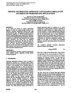
Filters are often composed of multiple layers, each of which is characterized by a porosity, an average pore diameter, and a retention function. We consider only single-layer filters in this work, though our simulator is capable of handling multiple layers. As the filter clogs, the volume of the void space decreases, leading to a decrease in the permeability. The pressure drop must then increase in order to maintain a constant mass flow rate throughout the filter. The large values of pressure required at the inlet may lead to damage of the metering pump, so the filter must be replaced once the pressure drop reaches a threshold value. The threshold value is set at 35e6 Pa in the simulator, which is comparable to existing industry thresholds [13]. A pressure drop curve for a filter with an initial porosity of 0.61 and an initial average pore diameter of 25.4 microns is given in Figure 2. 7
3.6
x 10
3.4
Pressure Drop (Pa)
3.2 3 2.8 2.6 2.4 2.2 2 1.8 1.6
0
20
40
60
80
100
120
Filtration time (hrs)
Figure 2: Pressure drop curve for representative filter More detailed information on the model can be found in [4, 7, 13].
4
American Filtration & Separations Society Annual Conference, May 19-22 (2008), Valley Forge, PA
3
MODELLING THE EXTRUSION FILTER PERFORMANCE
The optimization problem is formulated as Maximize (or Minimize)F (x), x ∈ Ω,
(1)
where F (x) represents the performance of the filter (e.g., lifetime), x is a vector of decision variables (filter parameter values), and Ω defines acceptable bound constraints on those parameters. We consider three problem formulations, each using a different measure of filter performance, resulting in different definitions of F (x). The performance of the filter is analyzed with respect to the filter parameters porosity, denoted by η, and average pore diameter, denoted by d p so that x = (η, dp ). The bound contraints are defined by the set Ω = {(η, dp ) : 0.4 ≤ η ≤ 0.65, 23 ≤ dp ≤ 40}.
3.1
F1 (x): Filter lifetime
The primary objective in our first problem formulation is to maximize the lifetime of the filter. A secondary, competing objective, is to minimize the amount of debris escaping the filter. This secondary objective is handled through the use of a barrier method. Taking into consideration the viewpoint of an engineer or production manager, we wish to define an acceptable bound on the escaped debris. This bound represents a level of debris that the manager would allow to make its way into the final product. Let b represent the bound, and let ξ(x) represent the total mass of debris that escapes over the lifetime of the filter. Naturally, we wish to construct the barrier function in such a way that ξ(x) is bounded away from b. In addition, the function should attain its minimum when ξ(x) = 0. These stipulations lead to the function B(ξ) =
ξ(x) , b − ξ(x)
(2)
which is defined on the half-open interval [0, b). We can see that B(ξ) → ∞ as ξ → b− . Likewise, B(ξ) → 0 as ξ → 0+ . Thus B(ξ) is minimized when ξ = 0 and grows without bound as ξ approaches b. Let t(x) represent the lifetime of the filter. Since we wish to maximize t(x), we will minimize its negative. This lends itself to the function F1 (x) = −t(x) + ρ1 B(ξ),
(3)
where ρ1 is a constant with units of hours. Note that, from the definition of B(ξ), we see that F1 (x) is not defined for values of x for which ξ(x) ≥ b. We handle such cases in a computational sense by setting F1 (x) to an unreasonably large value.
5
American Filtration & Separations Society Annual Conference, May 19-22 (2008), Valley Forge, PA
3.2
F2 (x) : Pressure drop across filter
As previously stated, we assume that the filter is replaced when the pressure drop reaches a certain threshold. For the second formulation, which is motivated by Figure 2, the primary objective is to minimize the maximum rate of change of the pressure drop across the filter. This offers a way of indirectly maximizing the lifetime of the filter. We retain the secondary objective of minimizing the total escaped debris. To quantify this primary objective,let pn denote the difference in pressure (in Pascals) across the filter at the nth timestep tn . The change in pressure between two successive timesteps can be written as pn − pn−1 ∆pn = , (4) tn − tn−1 which has units of Pascals per hour. If P = {∆p1 , ∆p2 , . . . , ∆pk }, where k is the total number of time steps, then clearly there is an αmin = sup P . Since x is fixed, it follows that there is associated with each value of x one and only one αmin . Hence, αmin can be written as a function of x. In order to incorporate the secondary objective, we keep the barrier function B(ξ) that was introduced in (2). This leads to the objective function F2 (x) = αmin (x) + ρ2 B(ξ),
(5)
where ρ2 is a constant with units of Pascals per hour. As with F1 (x), F2 (x) is defined only for values of x where ξ(x) < b; that is, where B(ξ) is defined. Computationally, this is handled in the same manner for both functions.
3.3
F3 (x) : Overall pressure change
As a variation of the pressure approach, we consider a linear estimate of the total change in pressure over the lifetime of the filter. Suppose the lifetime of the filter consists of N time steps. We measure the total change in pressure by constructing a line passing through the points (t 0 , p0 ) and (tN , pN ) (motivated again by Figure 2). A reasonable objective would be to minimize the slope of this line, which can be expressed as m=
pN − p 0 , tN − t 0
(6)
where m has units of Pascals per hour. Note that t0 = 0, and tN is simply the overall lifetime of the filter, so we have t = tN − t0 . Also note that we can easily express pN , p0 , and t as functions of x, which gives the objective function F3 (x) =
pN (x) − p0 (x) + ρ3 B(ξ). t(x) 6
(7)
American Filtration & Separations Society Annual Conference, May 19-22 (2008), Valley Forge, PA
Here B(ξ) is the barrier function defined in (2), and ρ3 is a constant with units of Pascals per hour. Once again, F3 (x) is defined for values of x where B(ξ) is defined and where t(x) 6= 0. The first case is handled as it was previously; the second can be neglected, since t(x) = 0 is impractical.
4
NUMERICAL RESULTS
We solve the optimization problem given by (1) using a MATLAB implementation of the implicit filtering algorithm developed by C.T. Kelley at North Carolina State University [10]. Implicit filtering is entirely derivative-free and is based on a quasi-Newton approach, which uses the objective function to build approximate gradients of F (x) and a secant-like method for the Newton-step [8, 12]. The advantage of implicit filtering is that the size of the finite-difference interval on which the gradient is approximated is decreased as the optimization progresses. This makes implicit filtering particularly effective for minimizing “noisy” functions; that is, functions that have a large number of local minima, which are not necessarily known in advance. By using large difference increments early in the optimization, the algorithm may avoid local extrema and close in on the global minimum. The algorithm requires a means to compute the objective function, a feasible initial iterate, and termination criteria either in the form of a function evaluation budget or a fixed number of times that the finite-difference stencil is reduced. Extensive numerical experiments were performed on all of the formulations of the objective function, using a variety of values for ρ. For the results presented here, we use ρ = 10 for F 1 (x) and ρ = 104 for F2 (x) and F3 (x). We used an initial iterate of x0 = (0.5, 25) and a budget of 60 evaluations of F (x). The allowable debris, b, was 8 × 10⁻⁵ kg. We present and discuss selected results from these tests. Table 4 contains results from the problem formulations. The data in the first column are the optimal values of (η, dp ) for each objective function. The data in the remaining columns provide the corresponding lifetime of the filter, αmin as described in Section 3.2, the mass of the escaped debris (ξ), and the slope of the secant line (m) for the overall pressure drop. Objective Function (η, dp ) F1 (0.6500, 26.9057) F2 (0.6500, 23.0000) F3 (0.6500, 28.6087)
t (hours) 76.0 67.8 79.3
αmin Pa/hr) 7.1749 6.8644 7.3072
(104
ξ (10−5
kg) 4.6591 3.3308 5.1403
m Pa/hr) 2.0407 2.2207 1.9747
(105
Table 1: A comparison of filter performance for F1 (x), F2 (x), F3 (x). All formulations result in identical values for porosity which lie on the upper bound constraint, but the values of pore diameter differ greatly between the three. In particular, note that F2 (x) offers the lowest values for both lifetime and escaped debris, F3 (x) offers the highest 7
American Filtration & Separations Society Annual Conference, May 19-22 (2008), Valley Forge, PA
values for both, and F1 (x) lies in the middle. It is apparent that F2 (x) is the most conservative of the three in terms of controlling the escaped debris, which may mean this formulation is most sensitive to the barrier. The expense is that the lifetime is significantly shorter than that of F1 (x) or F3 (x) More investigation is needed to explain why F2 (x) results in a pore diameter that is pushed towards the opposite bound constraint as the other two. It appears that the choice of pore diameter is highly dependent on the problem formulation. The varying results imply that the advantage of one formulation over another would be determined entirely by the preferences of a production manager, who must determine the relative importance of each objective. A more balanced solution may be reached by combining all three objectives into a single weighted objective function. In Figure 4 we show F1 (x) as it varies with the pore diameter and porosity value pairs sampled by the optimizer and we examine the corresponding lifetime of the filter for the various values of F1 (x). The figure on the left shows the various choices of (η, dp ) sampled by the optimizer. The porosity is clustered about η = 0.65 while the pore diameter varies more in an attempt to find the maximum. However, a majority of the design points are clustered near the best point found, which implies that the optimizer likely converged early within the function evaluation budget. The figure on the right shows that, as one would expect, F1 (x) varies nearly linear with the lifetime of the filter until the effects of the barrier term in F1 (x) become dominant. For design points where the filter lifetime is longer than 80 hours, we see there is a steep penalty for the amount of debris escaping the filter by the increase in the function value.
Objective Function F1(x) (hours)
Objective Function F1(x) (hours)
−25 −20 −40 −60 −80 0.7 35 0.6
30 25
Porosity
0.5
20
−30 −35 −40 −45 −50 −55 −60 −65 30
Pore Diam. (microns)
40
50 60 70 Filter Lifetime (hours)
80
90
Figure 3: Scatter plots of the value of F1 (x) versus (η, dp )(left) and lifetime (right). The same data is displayed in Figure 4 for F2 (x). In this case, the optimizer sampled a wider range of values for the porosity and the pore diameter prior to convergence, but we still see a cluster of points close to the minimum. The plot on the right demonstrates that this formulation 8
American Filtration & Separations Society Annual Conference, May 19-22 (2008), Valley Forge, PA
is slightly less sensitive to the barrier approach as there is less of a linear trend. 5
1.3
x 10
x 10
Objective Function F2(x) (Pa/hr)
Objective Function F2(x) (Pa/hr)
5
1.4 1.2 1 0.8 0.6 0.8 35 0.6
1.1 1 0.9 0.8
30 25
Porosity
1.2
0.4
20
0.7 0
Pore Diam. (microns)
20
40 60 Filter Lifetime (hours)
80
Figure 4: Scatter plots of the value of F2 (x) versus (η, dp )(left) and lifetime (right). Finally, we consider the results using the third objective function. As previously mentioned, the behavior of this function is somewhat similar to that seen for F1 (x). However, the optimizer sampled a wider range of design points in both η and dp . The optimal point identified for F3 (x) occurs at x = (0.6500, 28.6087), compared to x = (0.6500, 26.9057) for F 1 (x). In analyzing the second plot in Figure 4, we see that the slope defined in (6) is minimized when t is large, which is desirable. Also, we see in the first plot in Figure 4 that the optimizer samples more values for both the porosity and pore diameter in comparison to the other two. 5
4.5
x 10
x 10
Objective Function F3(x) (Pa/hr)
Objective Function F3(x) (Pa/hr)
5
5 4 3
2 0.7 35 0.6
3.5
3
2.5
30 25
Porosity
4
0.5
20
Pore Diameter (microns)
2 30
40
50 60 70 Filter Lifetime (hours)
80
90
Figure 5: Scatter plots of the value of F3 (x) versus (η, dp )(left) and lifetime (right). We also considered the same three formulations using an alternative derivative-free method, the DIRECT algorithm [6], for optimization and obtained essentially the same set of optimal 9
American Filtration & Separations Society Annual Conference, May 19-22 (2008), Valley Forge, PA
parameter sets for each formulation, implying that we have converged to at least a local (if not global) minimum.
5
CONCLUSIONS
A benefit of using a derivative-free sampling method for optimization is that intermediate function values can be used to analyze the behavior of the objective function and a wide variety of simulation methods can be used in a black-box fashion. Our goal is to better understand the measures of filter performance by investigating new objective functions and incorporating more decision variables. Previous work with the simulator indicates there is a huge benefit to using multi-layered filters, but we know of no organized study that has fully explored the design space associated with these more complicated structures. Optimization methods coupled with the simulator give us a mechanism to understand the interactions between our variables and deposition rates. We plan to extend our current work on single objective functions to give industrial partners an effective tool with which to reduce the operating costs associated with one of the components of fiber production.
References [1] http://www.clemson.edu/caeff. [2] R.B. Bird, W.E. Stewart, and E.N. Lightfoot. Transport Phenomena. Wiley, New York, 1960. [3] C.L. Cox, E.B Duffy, and J.B. von Oehsen. FISIM: The CAEFF integrated model for simulation of fiber and film processes. Plastics, Rubber, & Composites: Macromolecular Engineering, 33:426–437, 2004. [4] C.L. Cox, E.W. Jenkins, and P.J. Mucha. Modeling of debris deposition in a polymer extrusion filter. In Proceedings of PPS-21, Leipzig, Germany, June 2005. [5] D.D. Edie and C.H. Gooding. Prediction of pressure drop for the flow of polymer melts through sintered metal filters. Industrial and Engineering Chemistry Process Design and Development, 24:8–12, 1985. [6] D.E. Finkel. DIRECT Optimization Algorithm User’s Guide, March 2003. [7] K.R. Fowler, B. McClune, E.W. Jenkins, C.L. Cox, and B. Seyfzadeh. Design analysis of polymer filtration using a multi-objective genetic algorithm. Sep. Sci. Technol., 43(4):710– 726, 2008. [8] P.E. Gill, W. Murray, and M.H. Wright. Practical Optimization. Academic Press, 1982. 10
American Filtration & Separations Society Annual Conference, May 19-22 (2008), Valley Forge, PA
[9] D.C. Hookway. How to design your deep bed polymer filter. Filtration and Separation, pages 161–166, February 1996. [10] C.T. Kelley. Iterative Methods for Optimization. SIAM, 1999. [11] C.T. Kelley. User’s Guide for imfil Version 0.5, November 2005. [12] J. Nocedal and S.J. Wright. Numerical Optimization. Springer Series in Operations Research. Springer-Verlag, New York, 1999. [13] B. Seyfzadeh, D.A. Zumbrunnen, and R.A. Ross. Non-Newtonian flow and debris deposition in an extrusion filter medium. In Proceedings of Plastics – The Lone Star, pages 340–344. Society of Plastics Engineers, 2001.
11