a simulation study based on a non-adaptive randomized trial

MOX-Report No. 16/2017

Urn models for response-adaptive randomized designs: a simulation study based on a non-adaptive randomized trial

Ghiglietti, A.; Scarale, M.G.; Miceli, R.; Ieva, F.; Mariani, L.; Gavazzi, C.; Paganoni, A.M.; Edefonti, V.

MOX, Dipartimento di Matematica Politecnico di Milano, Via Bonardi 9 - 20133 Milano (Italy) [email protected]

http://mox.polimi.it

Urn models for response-adaptive randomized designs: a simulation study based on a non-adaptive randomized trial Andrea Ghiglietti1 , Maria Giovanna Scarale2,3 , Rosalba Miceli4 , Francesca Ieva5 , Luigi Mariani4 , Cecilia Gavazzi6 , Anna Maria Paganoni5 , and Valeria Edefonti2 February 21, 2017 1

2

Dipartimento di Matematica “F. Enriques” Universit` a degli Studi di Milano via Saldini, 50, 20133 Milano, Italy Laboratorio di Statistica Medica, Biometria, ed Epidemiologia “G. A. Maccacaro” Dipartimento di Scienze Cliniche e di Comunit` a Universit` a degli Studi di Milano via A. Vanzetti, 5, 20133 Milano, Italy 3 Unit of Biostatistics, Poliambulatorio “Giovanni Paolo II” IRCCS Casa Sollievo della Sofferenza Viale Padre Pio, 71013 San Giovanni Rotondo, Italy 4 Struttura Semplice di Epidemiologia Clinica e Organizzazione Trials Fondazione IRCCS Istituto Nazionale Tumori Via G. Venezian 1, 20133 Milano, Italy 5 MOX – Modellistica e Calcolo Scientifico Dipartimento di Matematica Politecnico di Milano via Bonardi 9, 20133 Milano, Italy 6 Struttura Semplice Dipartimentale di Terapia Nutrizionale Fondazione IRCCS Istituto Nazionale dei Tumori via G. Venezian, 1, 20133 Milano, Italy

Abstract Recently, response-adaptive designs have been proposed in randomized clinical trials to achieve ethical and/or cost advantages by using sequential accrual information collected during the trial to dynamically update the probabilities of treatment assignments. In this context, urn models - where the probability to assign patients to treatments is interpreted as the proportion of balls of different colors available in a virtual urn - have been used as response-adaptive randomization rules. We propose the use of Randomly Reinforced Urn (RRU) models in a simulation study based on a published randomized clinical trial on the efficacy of home enteral nutrition in cancer patients after major gastrointestinal surgery. We compare results with the RRU design with those previously published with the non-adaptive approach. We also provide a code written with the R software to implement the RRU design in practice.

1

In detail, we simulate 10,000 trials based on the RRU model in three setups of different total sample sizes. We report information on the number of patients allocated to the inferior treatment and on the empirical power of the t-test for the treatment coefficient in the ANOVA model. We carry out a sensitivity analysis to assess the effect of different urn compositions. For each sample size, in approximately 75% of the simulation runs, the number of patients allocated to the inferior treatment by the RRU design is lower, as compared to the non-adaptive design. The empirical power of the t-test for the treatment effect is similar in the two designs.

Keywords: non-adaptive trial design; Randomly Reinforced Urn model; Randomized trials; Response-adaptive randomization; Simulation study.

1

Introduction

In the statistical literature, urn models have been widely studied as mathematical tools to implement randomization in the context of clinical trials (e.g. see [1, 2]). These designs randomly assign those subjects that sequentially enter the trial to the treatment arms according to the color of the balls sampled from a virtual urn. Hence, the probability to assign a patient to a treatment arm is modelled by the proportion of the different types of balls in the urn. Recently, interest has been increased in the use of urn models for responses-adaptive designs, in which the probability to sample a ball of a certain type depends on the treatment performance observed on the subjects previously randomized [3, 4]. These designs are, therefore, able to achieve desirable statistical properties taking into account the ethical aspects of the clinical experiment (e.g. see [5]). A popular class of such designs is the Randomly Reinforced Urn (RRU) model, which has been introduced in [3] for binary treatment responses and extended in [6] to handle continuous responses. The main asymptotic results on the proportion of subjects assigned to the treatment groups by a RRU design have been established in [7] and [6]. For the purposes of this paper, we simply remind that a RRU design assigns patients to the superior treatment with a probability that converges to one as the sample size increases. For a complete overview on the RRU designs and its properties, we refer to [8]. Although the theoretical result of assigning most of the patients to the superior treatment is very attractive from the ethical point of view, the RRU design have rarely been implemented in clinical trials or in simulation studies based on a real set-up (e.g. see Chapter 12 in [9]). This may depend on some feasibility issues related to the practical implementation of adaptive designs in general. A key expertise is also required to implement urn models in clinical practice, which combines knowledge of the theoretical properties of urn models and experience in planning and running clinical trials. The substantial lack of dedicated software in standard statistical packages used in clinical practice is an additional issue that have prevented a wider use of RRU designs in this field. The aim of the current paper is to popularize the statistical and ethical advantages of the RRU design, and of urn schemes in general, and to promote their use in clinical practice through a dedicated code written in R [10]. In detail, we will simulate a large number of trials that follow the RRU model starting 2

from the real-life data collected in a (previously published) Home Enteral Nutrition (HEN) randomized trial [11], where a non-adaptive design was originally adopted. Comparing the performance of the RRU with that of the original nonadaptive design, we expect that the RRU design will: 1) assign fewer patients to the inferior treatment; 2) maintain similar inferential properties. This will turn out in an advantage in terms of both statistical performance and ethical responsibility. The paper is structured as follows. Section 2 provides some preliminary information on the HEN trial and its results [11], introduces the RRU model as a form of response-adaptive design, and describes how we carried out the simulations of the RRU design based on the original HEN data. Section 3 provides a comparison of the performance of the RRU versus the non-adaptive design in the simulation study based on the HEN data. Section 4 provides some suggestions on tuning parameters and the R codes for the implementation of a RRU design in the practice of randomized clinical trials. We conclude the paper with a Discussion (Section 5).

2 2.1

Materials and Methods A randomized controlled trial of home enteral nutrition versus nutritional counselling

The RRU model was here implemented in a simulation study based on results from a multicenter, controlled, open-label, two-parallel groups, randomized clinical trial conducted at the Fondazione IRCCS Istituto Nazionale dei Tumori (INT), Milan, Italy, and at the European Institute of Oncology, Milan, Italy, between December 2008 and June 2011 [11]. Malnutrition in gastrointestinal cancer patients is an independent risk factor for post-operative morbidity and mortality [12] and a prognostic factor for worst long-term outcome, especially after major surgery [13]. Therefore, the trial was primary aimed at investigating the effectiveness of enteral nutrition in limiting weight loss after home discharge from surgery, in comparison to nutritional counselling. The enrolled subjects were adult (> 18 years) patients with documented upper gastrointestinal cancer (esophagus, stomach, pancreas, biliary tract) who were candidates for major elective surgery and showed a preoperative nutritional risk score that indicated a potential benefit from any nutritional intervention. A random permuted block design (stratified for referring center) randomly assigned patients before discharge to receive either HEN to cover the basal energy requirement (experimental group), or nutritional counselling by an expert dietitian, including oral supplements only when needed (Control Group - CG), in a 1:1 ratio. The protocol allowed to remove HEN after two months from discharge if a weight gain ≥5% was reported and oral diet was regular and adequate. Therefore, the minimum treatment period in this trial was two months. The treatment effect was defined as the difference between the mean “weight change” (weight after two months - weight at baseline) in the HEN and nutritional counselling arms (primary end-point). The total sample size required to detect a statistically significant treatment effect was of 140 patients (70 per arm). The sample size was calculated with α = 5% (two-sided) and power 1 − β = 80% under the following assumptions derived from a previous pilot

3

study conducted at INT: baseline standard deviation of the weight distribution equal to 10 Kg, normality and homogeneity of weight variances across times of assessment and arms, 5 Kg of expected difference in the two-months mean weight change of treated versus control patients, and a correlation coefficient of 0.5 between baseline and two-months weights. The planned efficacy analyses included one interim and one final analysis, with the interim analysis to be carried out when half of the patients had been followed for at least two months. In order not to exceed an overall type I error of 5%, the nominal significance level required by each analysis for the evaluation of efficacy was 2.94%, according to the Pocok’s procedure [14]. The main analysis on the primary end-point was conducted with a univariate ANOVA including treatment as the main effect, after checking that standard ANOVA assumptions were satisfied. In total, 79 patients were initially randomized; however, as 11 patients had a missing two-months weight, the final analysis was performed on 68 patients, of which 33 patients were allocated to the HEN group and 35 to the CG. The main result of the primary end-point analysis was that the mean weight loss in the patients undertaking the HEN treatment was significantly lower than that in the CG, with a treatment effect estimated by the corresponding ANOVA model coefficient (95% confidence interval) of 3.2 (1.1-5.3) and a p-value from the corresponding two-sided t-test equal to 0.31% < 2.94%. For this reason, the trial was stopped at the interim analysis and results from this analysis were published in [11]. So, the HEN was found to be the superior treatment in this trial.

2.2

Randomly Reinforced Urn design

We briefly introduce a RRU model for continuous responses to two treatments [6], which has been implemeted in accordance with the design characteristics of the HEN trial. Consider a group of patients that sequentially enters a trial and has to be randomly assigned to either treatment R or treatment W. To model this, we assume that, before subject i ≥ 1 enters the trial, we have a virtual urn with Ri−1 > 0 red balls and Wi−1 > 0 white balls. We indicate with (Ri−1 , Wi−1 ) the urn composition before subject i ≥ 1 enters the trial. We also set the initial urn composition balanced (i.e., R0 = W0 ), to reflect the 1:1 randomization. When subject i enters the trial, a ball is sampled from the virtual urn and he/she is assigned to treatment R if the sampled color is red (Xi = 1) or to treatment W if the sampled color is white (Xi = 0). When his/her response to the assigned treatment is ascertained, we indicate it by ξRi if the assigned treatment is R or by ξW i if the assigned treatment is W. The responses to each treatment are assumed independent and identically distributed. The urn is then updated by adding balls of the same color of the sampled one; in detail, the number of balls added to the urn is represented by the utility function u, which is a suitable positive monotone increasing function of the response observed on subject i. Formally, the urn composition is updated as follows:   Ri = Ri−1 + Xi u(ξRi ) (1)  Wi = Wi−1 + (1 − Xi )u(ξW i ), 4

where we called ’reinforcement’ the quantities u(ξRi ) and u(ξW i ). The updating rule in (1) implies the single responses are available before the next patient enters the trial. In the case of ’delayed responses’, we propose here a variant of the previous design in the same spirit of [15]: the urn updating is based only on those responses that were available during the time interval between the arrivals of subject i and i + 1. Formally, for any i ≥ 1, let us denote by Ai the set of patients whose responses to treatments are available before subject i arrives. Then, the urn composition is updated as follows: P   Ri = Ri−1 + k∈(Ai+1 \Ai ) Xk u(ξRk ) (2) P  Wi = Wi−1 + k∈(Ai+1 \Ai ) (1 − Xk )u(ξW k ),

where (Ai+1 \ Ai ) refers to those subjects whose responses are available during the time interval between the arrivals of subject i and i + 1. In case of not delayed responses, (Ai+1 \ Ai ) = i, and hence (1) and (2) are equivalent. It follows from the RRU design definition that the probability to assign a subject i to the treatment R is the proportion of red balls in the urn at the moment of his/her entrance in the trial: P(Xi = 1|Ri−1 , Wi−1 ) =

Ri−1 , Ri−1 + Wi−1

(3)

where the right hand side of the formula indicates the urn proportion at time i − 1. Hence, the sequence {Xi ; i ≥ 1} of the subject assignment indicators is composed by conditionally Bernoulli random variables. In addition, it is worth noting that the urn proportion changes as far as a new response is made available; as a consequence, the probability to assign any new subject to one treatment or to the other depends on the treatment performance, in accordance with other response-adaptive designs. Pn Now, define NR (n) = i=1 Xi as the number of subjects assigned to treatment R among the first n patients enrolled in the trial and NW (n) = n − NR (n) as the number of subjects assigned to W. The main asymptotic result of the RRU design is that the proportion of subjects assigned to the superior treatment converges to one, as the sample size increases to infinity. Formally, denoting by mR := E[u(ξR1 )] and mW = E[u(ξW 1 )], from [6] we have that ( NR (n) a.s. 1 if mR > mW , → (4) n 0 if mR < mW . Hence, the RRU design asymptotically targets the superior treatment R. As a consequence, we expect that, in principle, a RRU design assigns a lower number of subjects to the inferior treatment with a higher probability, as compared to a non-adaptive design.

2.3

Simulations of Randomly Reinforced Urn designs

In this subsection, we describe how we simulated the RRU design starting from the HEN trial data and how we derived the results for comparing the RRU design with the non-adaptive one. We considered the following main steps: 5

(i) using the HEN trial dataset [11] described in Subsection 2.1: (1) we estimated the parameters of the Gaussian distribution of the responses to the HEN group; (2) we estimated the parameters of the Gaussian distribution of the responses in the CG; (3) we computed the empirical distribution of the difference between arrival times of consecutive subjects; (ii) we simulated N independent trial samples based on the RRU model; for each sample, responses to both treatments and intervals between arrival times were randomly generated from distributions introduced in point (i); (iii) we computed from these N trials: (1) the empirical distribution of the number of subjects assigned to the inferior treatment W; (2) the empirical power of the corresponding t-test. The previous steps are detailed in the following. To start, we considered three alternative set-ups of trial sample sizes equal to: (a) n = 58; (b) n = 68; (c) n = 78, where the total sample size 68 of the HEN trial (Section 2.1) was used as the reference set-up and we moved ±15% from that to get other two reasonable sample sizes. For each set-up, we performed N = 10, 000 simulations of independent trials based on the RRU design: in each run we have a virtual urn to be sampled and reinforced as described in Subsection 2.2. Formally, we denote by (Rij , Wij ) the urn composition and by Rij /(Rij + Wij ) the urn proportion in simulation j = {1, .., N } at time i ∈ {1, .., n}. All the urns start with the same (fixed) initial composition, i.e. (R0j , W0j ) = (R0 , W0 ) for any j = {1, .., N }. Then, the urn composition (Rij , Wij ) is updated as in (2):  j P j j j   Ri = Ri−1 + k∈(Aj \Aj ) Xk u(ξRk ) i+1

  Wj = Wj + i i−1

P

i

k∈(Aji+1 \Aji ) (1

j − Xkj )u(ξW k ),

j j j where Xkj is a Bernoulli random variable with parameter Rk−1 /(Rk−1 + Wk−1 ) j and the set Ai here includes all the patients who arrived two months earlier than subject i. Indeed, in the HEN trial, responses were available only two months after treatment administration. In addition, as normality assumptions in the original data were not rejected (see Subsection 2.1), responses to both treatments were generated as independent Gaussian random variables with arm-specific means and variances computed using the HEN dataset and given by: mR = −0.315 and σR = 3.868 for treatment R (HEN group), mW = −3.571 and σW = 4.789 for treatment W (CG). Formally, we generated the following quantities:

6

j j 2 (1) ξR1 , .., ξRn ∼ N (mR , σR ) potential responses to treatment R (HEN group); j j 2 (2) ξW 1 , .., ξW n ∼ N (mW , σW ) potential responses to treatment W (CG), j j where either ξRi or ξW i is observed, as each subject just receives one treatment. We also randomly generated the potential arrival times from the corresponding empirical distribution in the HEN dataset. For any sample size n (cases (a)-(b)-(c)) and any simulation j = {1, .., N }, we finally reported: P j (1) the number of patients NW (n) = (1 − Xij ) assigned to the CG, known to be the inferior treatment in the HEN trial (Subsection 2.1);

(2) the result Inj ∈ {0, 1} of the t-test for equal mean changes at level α = 0.05 (corresponding to the treatment coefficient in the ANOVA model): Inj = 0 if the test does not reject H0 , while Inj = 1 if the test rejects H0 . j It is worth noting that NW (n) (and consequently NRj (n)) typically differs across simulations, because the urn processes are independent and the subjects are allocated to the treatments depending on the urn-specific path of colors of the sampled balls. We also estimated the power of the t-test the N simulated P from j trials referring to the empirical power 1 − βˆ = N −1 N I . j=1 n Without loss of generality, we set the u function as: u(x) = (x + 20)/40. Since in the HEN trial the response values, x, range in the interval (−20, 20), this function was chosen to map linearly our simulated responses, x, in (0, 1). We also assumed the initial urn composition to be R0 = W0 = 1 (i.e. one ball of each color initially put into the urn). However, we carried out a sensitivity analysis to assess the effect of different initial urn compositions for the different total sample sizes available. In detail, we considered the cases: R0 = W0 = 5 or R0 = W0 = 10. To carry out the comparison with the non-adaptive design, we calculated the number of subjects allocated to the inferior treatment when the non-adaptive design was assumed. Let us denote this by nW . In case (b) (reference setup: n = 68), nW was known to be equal to 35, as in the HEN trial 35 out of 68 subjects were allocated to the inferior treatment. In addition, we have to estimate nW in cases (a) and (c). In case (a) (n = 58), we built several (≃ 10, 0000) subsamples of size 58 from the original HEN sample of total size 68; we estimated nW as the mean number of subjects allocated to the CG across the available samples of size 58. To estimate nW in case (c) (n = 78), we applied a proportin similar to that found in (b) on the 78 available subjects of this case. The corresponding nW were equal to 29 for case (a) and 38 for case (c). The empirical power of the adaptive design was compared with the theoretical power of the non-adaptive t-test which was computed assuming that the true difference of the mean weight changes between the two arms is equal to the value obtained in the HEN trial. All the analyses have been performed using a specialized code (available upon request from the authors) within the framework of the open-source statistical software R [10].

7

n 1 (a) 58 (b) 68 (c) 78

st

quartile 19 22 25

NW (n) Mean Median 25.6 25 29.6 29 33.6 33

3

rd

quartile 31 36 41

nW

1−β

1 − βˆ

29 35 38

0.88 0.92 0.94

0.83 0.88 0.92

Table 1: Summary statistics (1st and 3rd quartiles, mean, and median) of the empirical distribution of the number of subjects assigned to the inferior treatment, NW (n), and ˆ of the t-test for equal mean weight changes (corresponding empirical power, 1 − β, to the treatment coefficient in the ANOVA model) for the different sample sizes n in the Randomly Reinforced Urn design, in comparison with the corresponding results for the non-adaptive design, nW and 1 − β. We reported in bold typeface the results obtained with the same sample size of the original Home Enteral Nutrition trial. The initial composition of the urns in all simulations was set at: R0 = W0 = 1.

3

Results

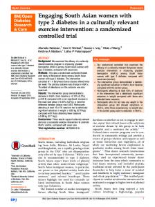
In this section we show the performance of the simulated RRU trials based on the HEN data. Table 1 shows some descriptive statistics of the empirical distribution of the number of subjects assigned to the inferior treatment, NW (n), ˆ for the different sample sizes n and the empirical power of the t-test, 1 − β, and a fixed initial urn composition R0 = W0 = 1, in comparison with the corresponding results for the non-adaptive design, nW and 1 − β. For all sample sizes under consideration [cases (a)-(b)-(c)], the mean and the median of NW (n) were smaller than nW , the number of subjects assigned to the inferior treatment by the non-adaptive design. It follows that the RRU design provided 50% of probability (or more) to assign fewer subjects to the inferior treatment, as compared to the non-adaptive design. Although higher than nW for all the sample sizes considered, the third quartile of NW (n) in the RRU design was very close to nW for any n under consideration. In addition, the obtained values for the t-test empirical power under the RRU design were close, but slightly smaller than, the corresponding power values derived in the non-adaptive design. Further information on the distribution of NW (n) is provided by the boxplots reported in Figure 1. For any sample size, the median of NW (n) was below the dashed line indicating the number of subjects assigned to the inferior treatment by the non-adaptive design. Similarly, we confirmed that, although higher, the third quartile was closer than the median to the dashed line for the three cases under consideration. In addition, the probability that NW (n) was less than nW was close to 75% for any sample size under consideration. Finally, although mostly symmetric, the empirical distributions of the number of subjects assigned to the inferior treatment showed a high level of variability. This variability increases, as the total sample size increases. Table 2 shows the results of the sensitivity analysis to different initial urn compositions. Our analysis was robust with respect to the initial urn composition chosen. Indeed, the mean and median number of subjects allocated to the inferior treatment in the RRU design was still below the corresponding number of subjects in the non-adaptive design, for any n and fixed urn composition under consideration. In addition, as far as the number of balls initially inserted 8

100 80 60 40 20

20 0

(c) n=78

0

20

40

60

80

100

(b) n=68

0

40

60

80

100

(a) n=58

Figure 1: Boxplots of the number of subjects assigned to the inferior treatment (Control Group) in the three cases reported above each picture: (a) n = 58, (b) n = 68, (c) n = 78. The dashed line indicated the number of subjects assigned to the control group in the non-adaptive trial in the three cases.

into the urn increases, for fixed n, the medians increase and, with R0 = W0 = 10, they almost reached the number of patients assigned to the inferior treatment in the non-adaptive design, nW . The empirical power of the t-test was correspondingly higher than in the reference scenario of R0 = W0 = 1 for any n under consideration, thus making it almost identical to the empirical power in the non-adaptive design (see column 1 − β in Table 1). Similarly, as far as the number of balls initially inserted into the urn increases, for fixed n, the variability of NW (n) decreases and the adaptive design becomes closer and closer to the non-adaptive one.

4

Practical implementation of the RRU design

In the following, we give some technical details on how to implement a RRU design in the practice of clinical trials. The initial set-up at the trial start involves: • total sample size n; • initial urn composition (R0 , W0 ); • utility function u. We highlight that the implementation of the RRU does not require any theoretical support or add-on code for sample size calculation. We just suppose 9

Scenarios n R0 = W0 1 58 5 10 1 68 5 10 1 78 5 10

1

st

quartile 19 23 24 22 27 29 25 31 33

Results NW (n) Mean Median 25.6 25 27.4 27 27.9 28 29.6 29 31.7 32 32.6 32 33.6 33 36.1 36 37.3 37

1 − βˆ 3

rd

quartile 31 31 31 36 36 37 41 41 42

0.83 0.86 0.87 0.88 0.91 0.91 0.92 0.94 0.94

Table 2: Sensitivity analysis to different urn initial compositions with R0 = W0 : summary statistics (1st and 3rd quartiles, mean, and median) of the empirical distribution of the number of subjects assigned to the inferior treatment, NW (n), and empirical ˆ of the t-test for the combination of different available sample sizes n and power, 1 − β, urn initial compositions. We reported the reference scenario in bold typeface.

that the trial investigators have calculated a total sample size n according to some approach, including traditional non-adaptive techniques. There is no standard approach to choose the initial urn composition. However, a rule of thumb could be to set R0 and W0 such that: (i) their sum (R0 + W0 ) is similar to the mean number of balls added to the urn at any time a new response is available, and (ii) the initial proportion of balls in the urn, Z0 = R0 /(R0 +W0 ), may reflect the a priori belief on which treatment is superior: the better the treatment R, the higher is Z0 . In our simulation study, we always set R0 = W0 and therefore: Z0 = 0.5, meaning that we have no reason to believe a priori that one treatment is superior. In accordance with the equipoise principle, this proportion is typically set to Z0 = 0.5 in the clinical practice. The utility function, u, is, in principle, any positive monotone increasing function that maps the range of continuos responses into a positive bounded interval. For instance, in our simulation of the HEN trial, since the response values, x, range in the interval (−20, 20), we set u(x) := (x + 20)/40, in order to obtain reinforcements in (0, 1). The RRU design is practically implemented as follows: • information storing: The minimal set of information for implementing the RRU design may be collected in two database. In the former one, we store for each subject (in rows) the following variables (in columns): – subject ID; – date of entry in the study; – treatment assignment; – date of response; – response value. 10

In the latter one, we store for each date of subject response (in rows) the updated urn composition (R, W ) (in columns). In the first row, we have the randomization date of the first patient entered in the study and (R0 , W0 ). • subject randomization: Equation (3) is implemented in the following R function: new_subject