A SIMULATION STUDY ON DYNAMICS AND CONTROL OF A REFRIGERATED GAS PLANT Nooryusmiza Yusoff*, M. Ramasamy and Suzana Yusup Department of Chemical Engineering Universiti Teknologi PETRONAS 31750 Tronoh, Perak, Malaysia Abstract Natural gas has recently emerged as an important source of clean energy. Improving operational efficiency of a gas processing plant (GPP) may significantly increase its profit margin. This proves to be a challenging problem due to the time-varying nature of the feedstock compositions and business scenarios. Such fluctuations in operational and economic conditions are handled by employing advanced process control (APC). Reasonably accurate steady-state and dynamic simulation models of the actual plant are required for the effective implementation of APC. This paper deals with the development of such models. Here, a refrigerated gas plant (RGP), which is the low temperature separation unit (LTSU) of the GPP, is modeled under HYSYS environment. Calibration and validation of the steady-state model of the RGP are performed based on the actual plant data. A dynamic model is also built to act as a virtual plant. Main control philosophies of the virtual plant are reported in this paper. This virtual plant model serves as a platform for performing APC studies. Keywords Gas processing plant, dynamic simulation, control Introduction The operators of gas processing plants (GPPs) face many challenges. At the plant inlet, several gas streams with different ownerships are mixed as a feedstock to the GPP. As a result, the feedstock compositions vary continuously. The feedstock comes in two types: 1) feed gas (FG), and 2) feed liquid (FL). The FG may be lean or rich depending on the quantity of natural gas liquids (NGLs). Lean FG is preferable if sales gas (SG) production is the main basis of a contract scenario. On the other hand, rich FG and higher FL intake may improve the GPP margin due to the increase in NGLs production. However, this comes at the cost of operating a more difficult plant. The GPP needs to obtain a good balance between smooth operation and high margin. At the plant outlet, the GPP encounters a number of contractual obligations with its customers. Low SG rate and off-specification NGLs will result in penalties. Unplanned shutdown due to equipment failure may also contribute to losses. These challenges call for the installation of advanced process control (APC). A feasibility study on the APC implementation may be performed based on a dynamic model. This model acts as a virtual plant. This way, the duration of the feasibility study will be shortened and the risk of interrupting plant operation will be substantially reduced. Simulation based on the first principles steady-state and dynamic models have been recognized as a valuable tool in engineering. Successful industrial applications of the first principles simulation are aplenty. Alsop and
* Email:
[email protected]
Ferrer (2006) employed the dynamic model of a propane / propylene splitter in HYSYS to skip the plant step testing completely. DMCPlus was used to design and implement the multivariable predictive control (MPC) schemes in the real plant. In another case, Gonzales and Ferrer (2006) changed the control scheme of depropanizer column based on a dynamic model. The new scheme was validated and found to be more suitable for APC implementation in the real plant. Several refinery cases are also available. For examples, Mantelli et al. (2005) and Pannocchia et al. (2006) designed MPC schemes for the crude distillation unit (CDU) and vacuum distillation unit (VDU) based on dynamic models. The previous works above demonstrate that dynamic simulation models can be utilized as an alternative to the empirical modeling based on step testing data. This way, the traditional practice of plant step testing to obtain the dynamic response may be circumvented prior to designing and implementing MPC. Worries about product giveaways or off-specifications may then be a thing of the past. In addition, the first principles simulation model may also be utilized to train personnel and troubleshoot plant problems offline. In the current work, the steady-state and dynamic models of a refrigerated gas plant (RGP) are developed under HYSYS environment. The steady-state model is initially calibrated with the plant data. This is used as a basis for the development of the dynamic model of the RGP. Finally, the regulatory controllers are installed to stabilize the plant operation and to maintain product quality.
Figure 1: HYSYS process flow diagram of the RGP. Equipment’s abbreviation: E=heat transfer unit (non-fired); S=separator; KT=turboexpander; K=compressor; P=pump; C=column; JT= Joule-Thompson valve; RV=relief valve. Controller’s abbreviation: FC=flow; TC=temperature; LC=level; SRC=split range; SC=surge; DC=digital on-off; SB=signal block.
Simulation The refrigerated gas plant (RGP) is simulated under HYSYS 2006 environment (Figure 1). The feed comes from three streams 311A, 311B and 311C with the following compositions (Table 1). Table 1: Compositions of feed gas at different streams Component Methane Ethane Propane i-Butane n- Butane i-Pentane n-Pentane n-Hexane Nitrogen Carbon Dioxide
311A 0.8865 0.0622 0.0287 0.0102 0.0059 0.0003 0.0002 0.0001 0.0039 0.0020
311B 0.7587 0.0836 0.0535 0.0097 0.0194 0.0058 0.0068 0.0002 0.0043 0.0580
311C 0.6797 0.1056 0.0905 0.0302 0.0402 0.0121 0.0101 0.0028 0.0012 0.0276
The thermodynamic properties of the vapors and liquids are estimated by the Peng-Robinson equation of state. Details of the process description have been described by Yusoff et al. (2007). The steady-state RGP model has high degree of fidelity with deviation of less than 6% from the plant data. This is an important step prior to transitioning to dynamic mode. Once the steady-state model is set up, three additional steps are required to prepare the model for dynamic simulation. The steps are equipment sizing, specifying pressure-flow relation at the boundary streams and installing the regulatory controllers. In the first step, all unit operations need to be sized accordingly. Plant data is
preferable to produce a more realistic dynamic model. In HYSYS, an alternative sizing procedure may be used. Vessels such as condensers, separators and reboilers should be able to hold 5-15 minutes of liquid. The vessel volumes may be quickly estimated by dividing the steadystate values of the entering liquid flow rates from the holdup time. For a column, only the internal section needs to be sized. This is accomplished by specifying the tray/packing type and dimensions. The tray must be specified with at least the following dimensions: 1) tray diameter, 2) tray spacing, 3) weir length, and 4) weir height. For a packed column, there are a number of packing types to choose from. Most of the packing comes with the pre-specified properties such as void fraction and surface area. The minimum dimension need to be entered is the packing volume or packing height and column diameter. For heat exchangers, each holdup system is sized with a k-value. This value is a constant representing the inverse resistance to flow as shown in Equation 1 (Aspentech, 2006): F = k ∆P
(1)
where, F = flow rate k = conductance or reciprocal of resistance ∆P = frictional pressure loss, which is pressure drop minus static head The k-value is calculated using the converged solution of the steady-state model. For practical purposes, only one heat transfer zone is required for the simple cooler (E-102) and the air-cooler (E-106). The E-102 is supplied with the
duty obtained from the steady-state model and E-106 is equipped with two fans. Each fan is designed to handle 3600 m3/h of air at 60 rpm maximum speed. The simulation of cold boxes is more challenging as they are modeled as LNG heat exchangers. Sizing is required for each zone and layer. Again for practical purposes, the number of zones in the cold boxes is limited to three. In each zone, the geometry, metal properties and a few sets of layers must be specified. The overall heat transfer capacities (UAs) and k-values are estimated from the steady-state solution and specified in each layer. Equipment with negligible holdup is easily modeled. For example, the dynamic specification for a mixer is always set to ‘Equalize all’ to avoid backflow condition. The flows of fluid across valves are governed by an equation similar to Equation 1. Here, the k-value is substituted with the valve flow coefficient, Cv. The valve is sized with a 50% valve opening and 15-30 kPa pressure drop at a typical flow rate. The rotating equipment such as pumps, compressors and expanders may be simulated in a rigorous manner. The main requirement is the availability of the characteristic curve of the individual equipment. The characteristic curves need to be added at the ‘Rating-Curves’ page in order to enhance the fidelity of the dynamic model. An example of the characteristic curves for K-102 is illustrated in Figure 2. 10000 9000
7072 RPM 5725 RPM
8000
Head (m)
7000
4715 RPM Operating Point
6000 5000
Control Philosophies
4000 3000 2000 1000 0 4000
6000
8000
10000
12000
14000
16000
14000
16000
Actual Flow (m3/h)
(a) Head curve 100 90 80 70
Efficiency (%)
The compressors and turbo expanders may also be modeled based on the steady-state duty and adiabatic / polytropic efficiency specifications. For pumps, only the power and static head are required. This simplification is recommended to ease the transitioning from steady-state to dynamic mode or to force a more difficult model to converge easily. In the current work, K/KT-101 are modeled in this manner since their characteristic curves are unavailable. In contrast, K-102, P-101 and P-102 models are based on the characteristic curves. The second step in developing a dynamic model is to enter a pressure or flow condition at all boundary streams. This pressure-flow specification is important because the pressure and material flow are calculated simultaneously. Any inconsistency will result in the ‘Integrator’ failure to converge. In addition, the compositions and temperatures of all feed streams at the flowsheet boundary must be specified. The physical properties of other streams are calculated sequentially at each downstream unit operation based on the specified holdup model parameters (k and Cv). In the current simulation work, all boundary streams are specified with pressure values. The feeds enter the RGP at 56.0 barg. The exiting streams are the NGLs stream at 28.5 barg and the SG stream at 33.5 barg. The flow specification is avoided since the inlet flows can be governed by PID controllers and the outlet flows are determined by the separation processes in the RGP. The final step is the installation of regulatory controllers. In most cases, base-layer control is sufficient. However, more advanced controllers such as cascade, split range and surge controllers are also installed to stabilize the production. The discussion of the plant control aspects is the subject of next section.
7072 RPM 60 5725 RPM 50 40
4715 RPM Operating Point
30 20 10 0 4000
6000
8000
10000
12000
Actual Flow (m3/h)
(b) Efficiency curve Figure 2: The K-102 characteristic curves
The control of plant operations is important to meet product specifications and to prevent mishaps. Due to space constraints, only main control philosophies are discussed in this section. The first loop is the TC-101 PID controller as shown in Figure 1. The purpose of this loop is to control Stream 401 temperature and indirectly the plant overall temperature. This is accomplished by regulating the cooler duty, E-102Q through a direct action mode. Stream 401 temperature is set at 37 oC to prevent excessive FG condensation into the first separator (S-101). In the event of excessive condensation, the S-101 level is regulated by a cascade controller. The primary loop (LC-101) controls the liquid level in the separator, which is normally set at 50%. This is achieved by sending a cascade output (OP) to the secondary loop (FC-102). The FC-102 acts in reverse mode to regulate Stream 402 flow between 0 and 60 ton/h. The magnitude of RGP throughput is controlled by the pressure of second separator (S-102). The S-102 pressure is regulated by the inlet vanes of KT-101 and the by-pass Joule-Thompson (J-T) valve as per split range operation (SRC-101). For example, the S-102 pressure is remotely set by FC-101 to decrease from 52.1 to 51.7 bar
(SRC-101 PV) in order to increase the throughput from 280 to 300 ton/h (FC-101 SP). At the same time, the SRC101 OP increases from 37 to 40% opening up the KT-101 inlet vanes to 80% while keeping the J-T valve fully close. The schematic of this loop is illustrated in Figure 3, the SRC-101 split range set up in Figure 4 and the close-loop response to a throughput step up in Figure 5. Feed Gas
2.72 to 2.35 mole %. The downstream effects can be seen at both suction and discharge sides of K-102. Lowering the C-101 Ptop will reduce the K-102 suction pressure (Psuct) from 25.0 to 23.5 bar. Consequently, the K-102 speed needs to be increased from 5684 to 6352 RPM in order to obtain a discharge pressure of 33.7 bar. The increase in K-102 speed causes its discharge temperature (Tdisc) to also increase from 40.6 to 60.2 oC.
E-102
K-102 Psuct
E-103
E-101
K-102 Tdisc
S-101
FC
SRC 101
101
C-101 Ptop KT-101
To C-101
J-T
C2 mole fraction
S-102
K-102 speed
Figure 3: Plant throughput control C-101 Ttop
100
Figure 6: Effect of C-101 Top Pressure
OP (%)
80 60
KT-101
J-T valve
Conclusions
40
A simulation model of refrigerated gas plant (RGP) was successfully developed. The dynamics of the RGP was simulated based on a high fidelity steady-state model. The dynamic model can be used as a virtual plant for performing advanced process control (APC) studies.
20 0 0
4
8
12
16
20
SRC-101 Signal Output (mA)
52.1
300
52 SRC-101 OP
295
51.9
290
51.8 SRC-101 PV
285
51.7
FC-101 SP 280 275 0.0
51.6
10.0
20.0
30.0
40.0
50.0
51.5 60.0
Acknowledgment
40.5 40 39.5 39 38.5 38
SRC-101 OP (%)
305
SRC-101 PV (bar)
FC-101 SP (ton/h)
Figure 4: SRC-101 split range setup
37.5 37 36.5
Time (min)
Figure 5: Response to throughput step up
Another important controller is PC-101, which regulates the C-101 top pressure (Ptop) by varying the K-102 speed. This loop provides the means for changing the RGP operation from ethane (C2) to propane (C3) recovery mode or vice-versa. An example of the closeloop response to the change from C3 to C2 mode is shown in Figure 6. The C-101 overhead is initially at 24 barg and -83.0 oC. To recover more C2, the column pressure is decreased to 22 barg. If all else remain the same, this action causes the C-101 top temperature (Ttop) to reduce to -86.4 oC and C2 composition in the SG to reduce from
The financial support from the Universiti Teknologi PETRONAS is highly appreciated. References Alsop N. and Ferrer J.M. (2006). “Step-test free APC implementation using dynamic simulation”. AIChE Spring National Meeting, Orlando, Florida, USA. Aspentech (2006). “HYSYS 2006 Dynamic Modeling Guide”. Aspen Technology: Cambridge, MA, USA. Gonzales R. and Ferrer J.M. (2006). “Analyzing the value of first-principles dynamic simulation”. Hydrocarbon Processing. September, 69-75. Mantelli V., Racheli M., Bordieri R., Aloi N. Trivella F. and Masiello A. (2005). “Integration of dynamic simulation and APC: a CDU/VDU case study”. European Refining Technology Conference. Budapest, Hungary. Pannocchia G., Gallinelli L., Brambilla A., Marchetti G. and Trivella F. (2006). “Rigorous simulation and model predictive control of a crude distillation unit”. ADCHEM. Gramado, Brazil. Yusoff N., Ramasamy M. and Yusup S. (2007). “Profit optimization of a refrigerated gas plant.” ENCON. Kuching, Sarawak, Malaysia.