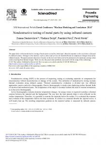
E-Journal of Advanced Maintenance Vol.3, No.1 (2011) 25-38 Japan Society of Maintenology
A Simulation Technique of Non-Destructive Testing using Magneto-Optical Film Huy Minh LE1, Jinyi LEE2,*, Sehoon LEE3 and Tetsuo SHOJI4 1, 2
Department of Control, Instrumentation and Robot Engineering, Chosun University, Gwangju, 501-759, Korea. 3 Research Center for Real Time NDT, Chosun University, Gwangju, 501-759, Korea. 4 New Industry Creation Hatchery Center, Tohoku University, Sendai, 980-8579, Japan. ABSTRACT An electro-magnetic field resulting from the application of a magnetic or electrical field to a metallic specimen is distorted due to the existence of a crack. The distribution of the magnetic field is changed by this distortion of the electro-magnetic field, and this change in the distribution can be visualized by the magneto-optical (MO) film in the magneto-optical nondestructive testing (NDT) method. The plane of a polarized light beam rotates when the beam is transmitted through an MO film because of the Faraday effect, a kind of magneto-optical effect. In this paper, an NDT simulation technique, which uses not only the Faraday effect, but also the change in the magnetic domains caused by an external magnetic field, the saturated magnetization effect, the effect of the magnetizer, the bias of the magnetic field and the temperature properties, is discussed. The simulation results are verified by comparing them to experiment results. KEYWORDS
ARTICLE INFORMATION
NDT, Crack, Faraday effect, Magneto-Optics, MO film, Leakage Magnetic Flux.
Article history: Received 15 December 2010 Accepted 28 April 2011
1. Introduction Nondestructive Testing (NDT) is a noninvasive technique used to determine the integrity, safety and maintenance of engineering systems. It makes assessments without doing harm, applying stress or destroying the test object. NDT is used widely in industrial areas such as aerospace, power generation, automotive, and railway. Some of the most widely used NDT methods are Ultrasonic Testing (UT), Radiographic Testing (RT), Electromagnetic Testing (ET), and Penetrant Testing (PT). Ultrasonic Testing (UT) uses high frequency sound energy in examinations and measurements. A UT system requires the use of a coupling liquid between the transducer and the specimen, making testing slow and tedious and making contact essential with the specimen. Radiographic Testing (RT) uses various types of expensive and cumbersome equipment. X-ray is transmitted through a specimen to send to a receiver on the opposite side. The adjustments to the test setup to carry out this transmittal are complicated and time consuming. Furthermore, this technique requires the operator to take specific precautions to avoid radiation hazards. Penetrant Testing (PT) requires a liquid penetrant or dry powder, which is applied to the surface of the specimen, as well as waiting time. Not only is this method is complicated, it is unable to evaluate the depths of cracks. Electromagnetic Testing (ET) is receiving much attention as a faster, implementation-easy and safe alternative to the other NDT techniques. ET induces electric currents or magnetic fields or both inside a specimen, whose electromagnetic response can be observed. Some common methods of electromagnetic testing are as follows: Magnetic Particle Testing (MPT), Magnetic Flux Leakage Testing (MFLT) and Eddy-Current Testing (ECT). Hall sensors, magnetic resistance (MR) [1, 2] sensors, and giant magnetic resistance (GMR) [3, 4] sensors are used as magnetic sensors to measure the distribution of a magnetic field in MFLT and ECT. Another kind of sensor is the Magneto-Optical (MO) sensor, which is used in MFLT [5] and ECT [6, 7]. With the MO sensor, the paint on specimen does not need to be removed because cracks *
Corresponding author, E-mail:
[email protected] ISSN – 1883 – 9894/11© 2011JSM and the authors. All rights reserved.
25
H. M. Le et al./ A Simulation Technique of Non-Destructive Testing usingMagneto-Optical Film
can be detected with no contact. The MO sensor has a wide detection area and high spatial resolution of magnetic domains, so it can inspect structures at high speed. An automated real-time method for evaluating MO images can improve detection ability, reduce human errors, and increase inspection accuracy and speed. Crack properties such the crack direction, size and shape need to be evaluated from the magnetic field distribution to determine the required maintenance time. A finite element method (FEM) can calculate the magnetic field. In FEM, the magnetic source, cracks and air are divided into either small elements or nodes according to crack size, and the simultaneous equations describing the electro-magnetic field at each element are solved [8]. Consequently, accuracy becomes proportional to time-consumption. Another numerical method uses a dipole model to analyze (DMA) [9~11] the magnetic field around cracks. In the DMA method, the crack is considered to be filled by dipoles with the dipole moments oriented opposite to the direction of the applied field. Thus, the intensity of the magnetic flux leakage (MFL) at a point outside the specimen is the sum of the intensities of the magnetic fields generated by these dipoles at the same point. MFL around cracks, which is calculated in DMA, can be used to model a crack easily. In this paper, we provide a simulation software using DMA to model cracks. Also, the limitation of and solutions by the software are discussed by comparing with them with the experimental results, which were obtained by using the MO sensor.
2. Principles 2.1.
Faraday effect and Magneto-Optical Sensor
The Faraday effect, a magneto-optical effect, is the interaction between light and magnetic field in a medium. When the polarized light beam is transmitted through a film (Magneto-Optical Film, MOF), the polarized plane of the light is rotated by an angle called the Faraday angle as shown in Fig. 1(a). This angle is proportional to the Verdet constant V, intensity of magnetization B, and the thickness of MOF t, as described by the equation (1) [12, 13]: (1)
θF= VBt
L-rotation (anticlockwise) when the direction of propagation and magnetization direction are parallel. R-rotation (clockwise) when the direction of propagation and magnetization direction is anti-parallel.
(a)
(b)
Fig. 1. (a) The Faraday effect and (b) the structure of magneto-optical film
An MO sensor contains an MO film (GdBi)3(FeAl)5O12 , which is grown on a substrate (GdCa)3(MgZrGa)5O12 and a vaporized aluminum reflecting film as shown in the Fig. 1(b). The Faraday rotation is almost doubled in this reflection-type optical system [14]. 2.2.
The change in the magnetic domains cause by an external magnetic field
The rotation angle and the direction of the Faraday angle are affected by the strength and direction of magnetization as indicated by equation (1). Usually, Verdet constant, V and thickness of ISSN – 1883 – 9894/11© 2011JSM and the authors. All rights reserved.
26
H. M. Le et al./ A Simulation Technique of Non-Destructive Testing usingMagneto-Optical Film
MOF, t are constants. Therefore, the strength and direction of the magnetization can be estimated by estimating the rotation angle. In addition, the magnetic domains of an MOF have only two directions, vertical, up and down to the plane of the MOF because of magnetic anisotropy. Therefore, the polarized light beam is rotated at a clockwise angle (θF) and anticlockwise angle (-θF) as shown in Fig. 2(a). Then the Analyzer obtains the electrical field of the light EB= Ecos(δ-θF) and ED= Ecos(δ+θF), where E is the electrical field of the transmitted light, and EB, ED are the electrical fields of +θF and –θF , respectively, and δ is the angle between the polarizer and analyzer (Fig. 2(a)). Since EB> ED, the MOF has alternating bright areas and dark areas. If there are no cracks on a specimen, the ratio of the bright area and dark area would be the same; if there are cracks on a specimen, the magnetic field around the cracks would be different from that in no-crack area, so the domain widths are changed. Therefore, cracks can be observed by using a polarizing optical system (Fig. 2(b)). Also, the domain width of a MOF is approximately 3-50 μm without a magnetic field, which means smaller cracks can be detected by using smaller magnetic domain widths of an MOF. (b)
(a)
Fig. 2. Effect of MOF
2.3.
Saturated magnetization of Magneto-Optical element (b)
(a)
Fig. 3. Saturated magnetization effect
As mentioned in the structure of an MOF, the MOF has a reflecting film which reflects the light from the polarizer. The reflected light will form an image on the MOF, including black and white colors according to the intensity of the reflected light. The intensity can be described by the following equation which describes the ratio of bright area and dark area [14]: 1 2
cos δ
θF
cos δ
θF
(2)
ISSN – 1883 – 9894/11© 2011JSM and the authors. All rights reserved.
27
H. M. Le et al./ A Simulation Technique of Non-Destructive Testing usingMagneto-Optical Film
where H( 0), I decreases, the width of the bright domain decreases, and 8 ), as in case ○ 1 , the dark and bright the width of the dark domain increases. When B= 0 (case ○ 9 (B< 0, H= -HS), the direction of magnetic field is inversed, and I domain are equal. In the case of ○ δ θF . There is only the dark domain. is minimum, 2.4.
Magnetization of a specimen
(a)
(b)
(c)
(d)
Fig. 4. Several magnetic methods; (a) yoke type magnetizer, (b) cross type magnetizer, (c) vertical type magnetizer, (d) sheet type induced current (STIC)
An MOF has dark or bright areas depending on the direction of magnetization. So, if we control the direction of magnetization, the dark and bright domains can be changed. When the direction of magnetization is horizontal which is induced by a yoke type magnetizer (Fig. 4(a)) [15], the MOF shows dark and bright domain continuously at the both side of a crack. Because of the large MFL around a crack, the areas of the domains are larger than those for a no-crack area. If the length of a crack is parallel to the magnetization direction, the MFL is minimized and the crack becomes difficult to inspect. In this case, a cross type magnetizer is a good solution (Fig. 4(b)). A cross type ISSN – 1883 – 9894/11© 2011JSM and the authors. All rights reserved.
28
H. M. Le et al./ A Simulation Technique of Non-Destructive Testing usingMagneto-Optical Film
magnetizer includes of two magnetic fields (induced by coil 1 and coil 2) that are perpendicular each others [16]. Another method uses a vertical magnetic field (Fig. 4(c)) [15]. The value of a vertical magnetic field can be controlled by the value of the input current in the coils. If the magnetic density in no-crack area (BZ, base) is slightly larger than the saturated magnetic density of the MO sensor (BS), the magnetic density in the crack area (BZ, crack) would be smaller than BS. Thus, the transaction of crack will occur. The direction of crack length does not affect detection ability, so this method can use for a thick specimen. A sheet type induced current (STIC) (Fig. 4(d)) [7] has been proposed for detecting subsurface corrosion and cracks in paramagnetic metals; this system is usually called the Magneto-Optical Imager (MOI) [6]. The alternative magnetic field induces a current in the induction foil (sheet type) on the specimen. Then, this sheet type induced current induces an eddy current around the crack in the specimen. This eddy current induces a magnetic field into the specimen which is perpendicular to the MOF. This magnetic field domain can be visualized by using MOI to observe the crack. 2.5.
Bias of the magnetic field
The MO sensor responds and forms an image only if the magnetic flux density exceeds a certain threshold value, Bs, which is a characteristic of the sensor. For example in MOI system, the eddy current (Fig. 4(d)) induces a small magnetic field, so a bias coil is used to induce an additional DC magnetic field (Fig. 5). This bias magnetic field permits adjustments to the MO sensor threshold and optimizes the sensor response to varying field strengths. This bias magnetic field is controlled by the DC bias current, so it’s easy to control the level of the sensor threshold. Fig. 6 shows the experiment results with hole type cracks using an MOI system. When we applied a (-) bias magnetic field, more accurate information about the cracks was obtained than when we had applied a (+) bias magnetic field. In addition, magnetic field background noises such as the earth’s magnetic field affected the quality of the MO sensor. Using a bias magnetic field, it was easy to reduce this background noise effect. Therefore, the sensitivity of the MO sensor can be adjusted by using a bias magnetic field. Ø6.36, d0.7
Ø8.4, d0.9
(-)bias
(+)bias
Fig. 5. Bias magnetic field
2.6.
Fig. 6. The change of MO threshold using bias magnetic field
Temperature properties
The NDT technique that can detect a natural crack in the high-temperature testing regime using an MOF was proposed [17]. Also, the behaviors of MOF in the low temperature regime have been studied. As shown in the Fig. 7, the domain width increases rapidly in the low temperature areas; therefore, the spatial resolution of MOF is decreased at low temperature. However, the spatial resolution of MOF is increased at high temperatures when the domain width is small. Fig. 8 shows the relation between the domain ratio and magnetic flux density for each temperature regime. The domain ratio is the ratio of bright and dark areas, which is approximately 50% without magnetic induction at room temperature. The expansion of the bright area or the increase of the domain ratio attributed to their linear relation with the increase of magnetic induction. The domain ratio rapid changes at the low temperature regime, so an MOF can saturate easily just with small magnetic induction at low temperatures. It means that an MOF has high sensitivity at low temperature. For a paramagnetic metal ISSN – 1883 – 9894/11© 2011JSM and the authors. All rights reserved.
29
H. M. Le et al./ A Simulation Technique of Non-Destructive Testing usingMagneto-Optical Film
specimen with small crack, the distortion of the magnetic field around the cracks is small, so they would have to be detected at low temperatures. The domain ratio changes at around the boiling point of water in Fig. 8. Therefore, the cracks on a specimen at several hundred degrees centigrade can be detected using an MOF submerged in distilled water near the boiling point. Then, the crack can be evaluated using the MOF at any temperature.
Fig. 7. Average domain width depends on temperature
2.7.
Fig. 8. Domain ratio due to the magnetic flux density
Simulation technique
(a)
(b)
Fig. 9. Dipole model in the case of (a) horizontal magnetization and (b) vertical magnetization
Fig. 9(a) shows the dipole model and coordinate system for the case of horizontal magnetization. The XY plane is represented on the surface of the specimen, the Y-direction is parallel with the length direction of the crack, the magnetization direction is in the X-direction, and the Z-direction is presented as the vertical direction to the surface of specimen. DMA assumes that magnetic charges exist on both walls of a crack. The magnetic charge of area (at the right wall in Fig. 9(a)) is . This magnetic charge induces a magnetic flux intensity at point r(x, y, ISSN – 1883 – 9894/11© 2011JSM and the authors. All rights reserved.
30
H. M. Le et al./ A Simulation Technique of Non-Destructive Testing usingMagneto-Optical Film
z) is
. The vertical directional components of the MFL in the Z-direction, is
. The total magnetic flux intensity at point r(x, y, z) which is induced by magnetic charges on the two walls of the crack can be described [10, 11]: /
4 4
/
/2
/
/
/
/2
/
(4)
where, m, , lc, wc, dc and z are the magnetic charge per unit area, permeability of the specimen, and the length, width, depth of the crack and the lift-off, respectively. Fig. 9(b) shows the dipole model and coordinate system in the case of vertical magnetization. The coordinate system is represented in the case of horizontal magnetization, as well. We assumed following: the size of the specimen is larger than the size of the crack ( , ; , are length and width of specimen), uniform magnetic charge per unit area, m on the surface of specimen and at the bottom of the crack; and to be distributed on the whole surface of the specimen of width wS and length lS (the magnetic flux intensity would be HZ, all). The crack area with width wc and length lc, actually, has no magnetic charge (the magnetic flux intensity would be HZ, crack). At the bottom of this crack, m is assumed to be distributed over an area of width wc, and length lc , located at dc distance in ) shown in Fig. 9(b), the Z-direction (the magnetic flux intensity would be HZ, under). For an area ( the magnetic flux intensity at point r(x, y, z) in the Z-direction can be expressed by equation (5) [9, 10]. From these suppositions, the distribution of the overall magnetic field can be calculated by equation (6). Furthermore, when the crack is moved (x offset, y offset) and rotated by θc from its center on the XY plane, the crack position in the new plane XRYR (Fig. 10) can be expressed by equation (7) [18]. In the case of vertical magnetization, the Hz does not change. But in the case of horizontal is changed to cos . magnetization, the
Fig. 10. Model of crack and its relocated position
/
4 ,
,
,
,
(5) (6) (7)
ISSN – 1883 – 9894/11© 2011JSM and the authors. All rights reserved.
31
H. M. Le et al./ A Simulation Technique of Non-Destructive Testing usingMagneto-Optical Film
Fig. 11(a) shows the distribution of HZ for the case of θc= 00 with horizontal magnetization. The crack size is wc= 1 mm, lc= 10 mm, dc= 1 mm, lift-off z= 1 mm, m/4 = 1 in the area x= [-10:10] mm , y= [-10:10] mm. For the case of θc= 900, we just need to exchange wc and lc as shown in Fig. 11(b). Fig. 11(c) shows the distribution of HZ for the case of θc= 00 with vertical magnetization. The = 1 in the area x= [-10:10] crack size is wc= 1mm, lc= 10 mm, dc= 1 mm, lift-off z= 1 mm, m/4 mm, y= [-10:10] mm, and the specimen size is width ws and length ls. For the case of θc= 900, we just need to exchange the wc and lc, as shown in Fig. 11(d). Magnetization direction
Magnetization direction
(b) z
(a) z
y
x
y
x (d)
(c)
z
z
Magnetization direction
x
Magnetization direction
y
x
y
Fig. 11. Distribution of Hz in the case of (a), (c) θc= 00 and (b), (d) θc= 900 (a), (b) horizontal magnetization; (c), (d) vertical magnetization (a)
(b)
Fig. 12. Image processing. (a) horizontal magnetization, (b) vertical magnetization
The software consisted of Visual Basic 6.0 and a 3-D tool (CW3DGraph 6.0 of Measurement Studio by National Instruments Co.). The crack was visualized in 3-D, so the surface of the specimen and depth of the crack were expressed by the XY plane and Z axis of the graphic tool, respectively. Rectangular type, triangular type, elliptical type and step type cracks were simulated in the software. Also, multiple, complex cracks were expressed by superposing several graphs, which had the same XY plane and the same scale of the Z axis. These superposed graphs showed the different shapes and sizes of the cracks. Thus, the distribution of MFL can be calculated by using the above equations from ISSN – 1883 – 9894/11© 2011JSM and the authors. All rights reserved.
32
H. M. Le et al./ A Simulation Technique of Non-Destructive Testing usingMagneto-Optical Film
Eq. (3) to Eq. (7) when multiple complex cracks are located at any position and direction on the specimen. However, the z in each equation expresses the lift-off, the distance between the specimen surface and the sensor. Depending on the MFL distribution around a crack, different domains appear on MOF. In the case of horizontal magnetization, the magnetic domain around a crack is larger than that in no-crack area. Hence, the bright and dark domains appear large around a crack, and smaller stripe domains appear far from a crack. In the case of vertical magnetization, the magnetic domain in a no-crack area is saturated by MOF. Only the magnetic intensity in a crack area is lower than the saturated magnetic intensity of MOF. So the MOF shows a dark domain in a crack area and a bright domain in a no-crack area. The software has three colors, bright for H H , dark for H H , and dusky for -HS< HZ< HS. These colors appear in the case of horizontal magnetization as shown in Fig. 12(a) [18]. The bright color is around the dusky color which displays a crack in the case of vertical magnetization as shown in Fig. 12(b). Furthermore, the parameters such as magnetic charge per unit m, permeability of specimen , saturated magnetic intensity of MOF HS, bias magnetic intensity Hb, and the temperature regime T were introduced in the software. When bias magnetic intensity is applied, the total magnetic intensity distribution is HZ + Hb. The temperature affects to the value of saturated magnetic intensity of MOF HS as shown in Fig. 8 and the spatial resolution of MOF as shown in Fig. 7. The spatial resolution of the MOF was expressed as the meshing number of the 3-D graphic. So, when the temperature T changes, the HS and meshing number are changed automatically. Thus, we can simplify the principles in Table 1. Table 1 Relation between the real condition and the simulation
Real Condition Lift-off Bias magnetic field Saturated magnetic field of MOF
Magnetization direction
Temperature
Simulation z H H H Hs H Bright color for H Dark color for H H H Dusky color for H Two options in the software: 1. Vertical magnetization 2. Horizontal magnetization is affected by angle θc Changing the sensitivity of MOF (Hs) Changing the width of domain(meshing number of 3D graphic)
3. Experiments and discussion Table 2 Size of cracks Magnetization direction
Fig. 13. Cracks on specimen
ISSN – 1883 – 9894/11© 2011JSM and the authors. All rights reserved.
33
H. M. Le et al./ A Simulation Technique of Non-Destructive Testing usingMagneto-Optical Film
Fig. 13 shows a specimen of 250 x 250 x 5 mm in size, made of low carbon steel (SS41). Table 2 shows the rectangular cracks of different sizes with angels of θc= 00, 450, 600, 900. Cracks No. 5, No. 10, No. 15 and No. 20 are hole types, which were simplified as a square in the numerical analysis. The cracks were machined by using an electro-discharge machine.
Fig. 14. (a) yoke type magnetizer, (b) cross type magnetizer Table 3 Parameters of software using for horizontal magnetization
Table 4 Parameters of software using for vertical magnetization
Magnetization direction of yoke type magnetizer
Fig. 15. Simulation results with yoke type magnetizer
Fig. 16. Experimental results with yoke type magnetizer
Magnetic field was applied by using a yoke type magnetizer, as shown in Fig. 14(a). The yoke type magnetizer has 2 coils with each coil having 2000 turns. The two cores are 220 mm in height, and 150 mm in length with the distance between the cores of 250 mm. The 0.1 A direct current was supplied to each coil with the different direction each other. Figs. 15 and 16 show the simulation results and experimental results with the parameters in Table 3. The experimental results and simulation results were similar in the case of rectangular type cracks. As mentioned in the discussions on the principles, bright and dark area existed around cracks. The cracks with the angle θc= 00 (No. ISSN – 1883 – 9894/11© 2011JSM and the authors. All rights reserved.
34
H. M. Le et al./ A Simulation Technique of Non-Destructive Testing usingMagneto-Optical Film
1~No. 4 in Fig. 13) were easier to detect than the other cracks. On the other hand, the cracks with the angle θc= 900 (No. 16~No. 19 in Fig. 13) could not be detected because the magnetization direction was perpendicular with the length directions of cracks (in the case of θc= 00), and parallel with the length directions of cracks in the case θc= 900. In the case of θc= 450 and θc= 600, cracks were also detected. Detection ability reduced according on the increase of the angle θc. Also, detection ability increased according to the increase of the depth of crack as shown in No. 3, No. 8 and No. 13. However, in the case of hole type cracks, the simulation results are different from the experiment results because the hole type cracks were assumed as square type cracks in the numerical analysis software. The experiment results appeared the brightness was lighter on the left side and darker on the right side because the north magnetizer pole and south magnetizer pole were on the left and right sides of specimen, respectively. Magnetization direction 1
Fig. 17. Simulation results with cross type magnetizer (pair 1)
Fig. 18. Experimental results with cross type magnetizer (pair 1)
Magnetization direction 2
Fig. 19. Simulation results with cross type magnetizer (pair 2)
Fig. 20. Experimental results with cross type magnetizer (pair 2)
ISSN – 1883 – 9894/11© 2011JSM and the authors. All rights reserved.
35
H. M. Le et al./ A Simulation Technique of Non-Destructive Testing usingMagneto-Optical Film
The cross type magnetizer has 4 cores of 200 mm in height, 150 mm in width, and 250 mm in pole distance, as shown in the Fig. 14(b). Each core is wound by 2000 turns of coil. The horizontal and vertical magnetic fluxes are obtained after direct current is supplied to a pair of coils, which face each other. Figs. 17, 19 are the simulation results obtained with the parameters in Table 3. Figs. 18, 20 are the experiment results for input current of 0.1 A supplied to each pair of coils. When current was input to the pair of coils (pair 1) which was line on the left side and right side of the specimen, the horizontal magnetization from left side to right side (magnetization direction 1) occurred on specimen (Fig. 18). Only cracks No. 16~19 (Fig. 13) did not appear because theirs length directions were parallel with the magnetization direction. This result is the same with the results of the yoke type magnetizer above. By supplying current to another pair of coils (pair 2), which was in line on the back side and front side of specimen, we could obtain the horizontal magnetization from back side to front side of the specimen (magnetization direction 2) as shown in Fig. 20. Cracks No. 1~4 (Fig. 13) did not appear because their direction of length were parallel to the magnetization direction. But other cracks appeared by the same reasons that were discussed in yoke type magnetizer. However, in cases of No. 11~14 (Fig. 13), these cracks appeared more clearly in Fig. 19 than in Fig. 17 because their θc= 30o in Fig. 17 was changed θc= 60o in Fig. 19. Therefore, we can switch the input current between each pair of coils to detect both cracks of θc= 0o and θc= 90o. These simulation results were similar with the experiment results in Fig. 18 and Fig. 20. The information of cracks appeared but not clearly in No. 3, 4 (Fig. 13) in Fig. 20 and No. 17, 18 (Fig. 13) in Fig. 18 because of the magnetic induction effect between the two coil and the residual magnetic field in each coils. (a)
(b)
Fig. 21. (a) Simulation result and (b) experimental result with vertical magnetization
Fig. 21 shows the simulation result (a) and experimental result (b) in the case of vertical magnetization. A rectangular crack of 0.5 mm of width, 10 mm of length and 4 mm of depth on SS41 specimen was used. The yoke type magnetizer (Fig. 14(a)) was used to induce vertical magnetization with 0.17 A direct current supplied to two coils in the same direction. The parameters for simulation are shown in Table 4. In the both results, only the information of crack appeared. In the case of the simulation result (Fig. 21(a)), the information of crack appeared as dusky color, and the no-crack area appeared as bright color as mention in the principle discussions. The magnetic intensity in the crack area was HZ, crack, -HS< HZ, crack< HS and the magnetic intensity in no-crack area was HZ, no crack , HZ, no crack ≥ HS. In the experiment result (Fig. 21(b)), the crack appeared with dark color but not smoothly because of noises.
4. Conclusion Numerical analysis software using a dipole model and a Magneto-Optical Film was used to simulate the distribution of the magnetic flux around cracks. The software allowed 3-D visualization of the magnetic distribution around a crack or multi-complex cracks on specimen of different shapes, sizes, positions and length directions. The Faraday effect in MOF was integrated into the dipole model and in the software. The software supported user input of important parameters such as lift-off distance, magnetic charge per unit area, saturated magnetic intensity of MOF, bias magnetic intensity, ISSN – 1883 – 9894/11© 2011JSM and the authors. All rights reserved.
36
H. M. Le et al./ A Simulation Technique of Non-Destructive Testing usingMagneto-Optical Film
and temperature. Horizontal magnetization and vertical magnetization were implemented in the software. The software performance was determined by comparing the simulation results with the experiment results. Horizontal magnetization was induced by using a yoke type magnetizer, to detect cracks except the cracks whose direction of length were parallel with the magnetization direction. A cross type magnetizer was used to induce horizontal magnetization, to detect cracks in all direction. In the case of vertical magnetization, only the information about cracks was shown without the effect of crack direction.
Acknowledgement This research was supported by the MKE (The Ministry of Knowledge Economy), Korea, under the ITRC (Information Technology Research Center) support program supervised by the NIPA (National IT Industry Promotion Agency) (NIPA-2011-C1090-1121-0013). We are grateful for the supports.
References
[1] K.Kosmas, Ch. Sargentis, D. Tsamakis, E. Hristoforou, Non-destructive evaluation of magnetic metallic materials using Hall Sensors, Journal of Materials Technology 161 (2005), pp. 359-392. [2] Jin Tao, Que Peiwen, Tao Zhengsu, Development of magnetic flux leakage pipe inspection robot using Hall sensors, IEEE 2004, pp.325-329. [3] Johannes Atzlesberger, Bernhard Zagar, Magnetic flux leakage measurement setup for defect detection, Procedia Engineering 5 (2010), pp. 1401-1404. [4] Kataoka, Y., Wakiwaka, H., Shinoura, O., Leakage flux testing using a GMR line sensor and the rotating magnetic field, IEEE Vol.2 (2002) pp. 800-803. [5] J. Lee, H. Lee, T. Shoji, D. Minkov, Application of Magneto-Optical Method for Inspection of the Internal Surface of a Tube, Electromagnetic nondestructive evaluation (II), IOS Press, Amsterdam 1998, pp. 49-57. [6] J. Lee, J. Jun, J. Kim, Jaesun Lee, An application of a magnetic camera for an NDT system for aging aircraft, Journal of the Korean Society for Nondestructive Testing Vol. 30, No. 3, 06/2010. [7] Y. Deng at al., Characterization of magneto-optic imaging data for aircraft inspection, IEEE Vol. 42, No. 10, 11/2006, pp. 3228 - 3230. [8] J. Lee, J. Hwang, T. Shoji, J. Lim, Modeling of characteristics of Magneto-optical sensor using FEM and Dipole Model for Nondestructive Evaluation, Key Engineering Materials Vols.297-300 (2005) pp. 2022-2027. [9] M. Dutta, H. Ghorbel, K. Stanley, Dipole modeling of magnetic flux leakage, IEEE Vol. 45, No. 4, 2009, pp. 1959 - 1965. [10] J. Lee, S. Lyu, Y. Nam, An algorithm for the characterization of surface crack by use of dipole model and magneto-optic Non-Destructive inspection system, KSME 2000 Vol. 14, No. 10, pp. 1072-1080. [11] D. Minkov, J. Lee, T. Shoji, Improvement of the Dipole Model of a Surface Crack, Material Evaluation, Vol. 58, No. 5, pp. 661-666. [12] J. Lee, T. Shoji, D. Minkov and M. Ishihara, Novel NDI by use of Magneto-Optical Film, Journal of The Japan Society of Mechanical Engineers (A) 1998, Vol. 64, No. 619, pp. 825-830. [13] J. Lee, T. Shoji, Development of a Novel NDI System by use of Magneto-Optical Film, Proceedings of JSNDI Spring Conference (1997) pp. 185-188. [14] M. Ishihara, T. Sakamoto, K. Haruna, N. Nakamura, K. Machida, Y. Asahara, Advanced Magnetic Flux Leakage Testing System using Magneto-Optical Film, The Japanese Society for Non-Destructive Inspection, 45(4) (1996) pp. 283-289. [15] J. Lee, T. Shoji, D. Seo, Theoretical consideration of nondestructive testing by use of vertical magnetization and magneto-optical sensor, KSME Int J Vol.18 No. 4, pp 640~648, 2004. [16] J. Lee, J. Hwang, S. Choi, A study of the quantitative nondestructive evaluation using the cross ISSN – 1883 – 9894/11© 2011JSM and the authors. All rights reserved.
37
H. M. Le et al./ A Simulation Technique of Non-Destructive Testing usingMagneto-Optical Film
type magnetic source and the magnetic camera, KEM Vols. 321-323 (2006), pp. 1447-1450. [17] J. Lee et al., Non-destructive testing in the high-temperature regime by using a magneto-optical film, NDT&E International 41(2008) pp. 420-426. [18] J. Lee, J. Jun, J. Hwang, S. Lee, Development of numerical analysis software for the NDE by using dipole model, Key Eng Mat Vols. 353-358 (2007) pp. 2382-2386.
ISSN – 1883 – 9894/11© 2011JSM and the authors. All rights reserved.
38