1006
WEATHER AND FORECASTING
VOLUME 20
A Single-Station Approach to Model Output Statistics Temperature Forecast Error Assessment ANDREW A. TAYLOR
AND
LANCE M. LESLIE
School of Meteorology, University of Oklahoma, Norman, Oklahoma (Manuscript received 18 June 2004, in final form 11 April 2005) ABSTRACT Error characteristics of model output statistics (MOS) temperature forecasts are calculated for over 200 locations around the continental United States. The forecasts are verified on a station-by-station basis for the year 2001. Error measures used include mean algebraic error (bias), mean absolute error (MAE), relative frequency of occurrence of bias and MAE values, and the daily forecast errors themselves. A case study examining the spatial and temporal evolution of MOS errors is also presented. The error characteristics presented here, together with the case study, provide a more detailed evaluation of MOS performance than may be obtained from regionally averaged error statistics. Knowledge concerning locations where MOS forecasts have large errors or biases and why those errors or biases exist is of great value to operational forecasters. Not only does such knowledge help improve their forecasts, but forecaster performance is often compared to MOS predictions. Examples of biases in MOS forecast errors are illustrated by examining two stations in detail. Significant warm and cold biases are found in maximum temperature forecasts for Los Angeles, California (LAX), and minimum temperature forecasts for Las Vegas, Nevada (LAS), respectively. MAE values for MOS temperature predictions calculated in this study suggest that coastal stations tend to have lower MAE values and lower variability in their errors, while forecasts with high MAE and error variability are more frequent in the interior of the United States. Therefore, MAE values from samples of MOS forecasts are directly proportional to the variance in the observations. Additionally, it is found that daily maximum temperature forecast errors exhibit less variability during the summer months than they do over the rest of the year, and that forecasts for any one station rarely follow a consistent temporal pattern for more than two or three consecutive days. These inconsistent error patterns indicate that forecasting temperatures based on recent trends in MOS forecast errors at an individual station is usually not a good strategy. As shown in earlier studies by other authors and demonstrated again here, MOS temperature forecasts are often inaccurate in the vicinity of strong temperature gradients, for locations affected by shallow cold air masses, or for stations in regions of anomalously warm or cold temperatures. Finally, a case study is presented examining the spatial and temporal distributions of MOS temperature forecast errors across the United States from 13 to 15 February 2001. During this period, two surges of cold arctic air moved south into the United States. In contrast to error trends at individual stations, nationwide spatial and temporal patterns of MOS forecast errors could prove to be a powerful forecasting tool. Nationwide plots of errors in MOS forecasts would be useful if made available in real time to operational forecasters.
1. Introduction Statistical forecasting techniques have been used operationally by the National Weather Service (NWS) since 1968 to forecast various near-surface weather elements (Carter et al. 1989). These techniques include
Corresponding author address: Andrew A. Taylor, School of Meteorology, University of Oklahoma, Rm. 1310, 100 E. Boyd St., Norman, OK 73019. E-mail:
[email protected]
© 2005 American Meteorological Society
the “perfect prog” (PP) method (Klein et al. 1959) and model output statistics (MOS; Glahn and Lowry 1972). Both methods forecast meteorological variables using predictive equations generated via multiple linear regression. In creating the PP forecast equations, training input parameters are taken exclusively from observational data and climate data, whereas predictor training parameters for MOS equations are largely drawn from numerical weather prediction (NWP) model output. Both PP and MOS systems are capable of accounting for local effects that cannot be resolved by numerical models. In addition, both systems use model output
DECEMBER 2005
TAYLOR AND LESLIE
variables as predictors. However, because the PP equations are formulated from raw or analyzed observational data, forecast parameters from any numerical model may be substituted into them, whereas MOS systems should use model output generated by the model(s) from which the equations were developed as predictor data. The accuracy of PP forecasts is limited by the accuracy of the model forecast parameters that go into the equations (Carter et al. 1989). The very best PP equations developed from observational data will likely produce poor results when applied to model output. MOS has the advantage of being able to correct for certain consistent biases in numerical model predictions because its equations statistically, rather than physically, relate observed values to model forecast variables. A major limitation of MOS is that the use of model-based predictors has the undesirable effect of rendering MOS output sensitive to changes in the model formulation or the introduction of a new model. However, MOS consistently outperforms the PP method in predicting maximum and minimum temperatures due to its ability to account for some, but not all, systematic model inaccuracies and the inclusion of many predictors unavailable to the PP method (Klein and Glahn 1974). The MOS technique has been used with considerable success over the years to predict the evolution of numerous weather elements. For example, MOS has been used to forecast maximum and minimum temperatures (Klein and Hammons 1975; Jacks et al. 1990), synoptic weather types (McCutchan 1978), and marine fog probabilities (Koziara et al. 1983). The specific focus of this study is on maximum–minimum and 0000–1200 UTC temperature forecasts, produced by MOS systems from the Nested Grid Model (NGM; Phillips 1979) and the Aviation Model run [AVN, presently the Global Forecast System (GFS)] of the National Centers for Environmental Prediction (NCEP) Global Spectral Model (GSM) (Kanamitsu 1989). As the numerical models from which they are derived become more advanced, MOS temperature forecasts see steady improvement. For example, by the 1987–88 cool season (October– March), the mean absolute error (MAE) of MOS 48-h maximum temperature forecasts was lower than the MAE of 24-h forecasts from the early 1970s (Carter et al. 1989). Progress continues up to the present time, although at a slower rate. The 24-h MOS maximum temperature forecasts from both the NGM and AVN have an overall MAE of around 3°F (Dallavalle et al. 2004), representing a decrease of less than 0.5°F since the late 1980s. The MAE of 48-h forecasts is between 3.5° and 4°F, a decrease of around 0.5°F since the late 1980s.
1007
There are a number of different approaches to the verification of MOS temperature forecasts. Common measures of forecast bias and accuracy include the mean algebraic error (Klein and Glahn 1974), henceforth referred to as the bias, and the mean absolute error (MAE). Often, these statistics are calculated on a regional or national basis, thereby measuring the overall accuracy of and bias in MOS temperature forecasts. However, grouping large numbers of bias and MAE values together obscures some of the error characteristics of MOS temperature forecasts unique to particular stations. Bias and MAE statistics can be computed for each observing station, and that is the approach we take in this paper. Verification of temperature forecasts on a station-bystation basis has been employed by many researchers in the past (Klein and Hammons 1975; Brenner 1986; Carter et al. 1989) to discover error characteristics unique to individual locations. Brenner (1986) examined MOS minimum temperature forecasts for five cities in Arizona and found pronounced warm biases for each city. In addition, Carter et al. (1989) documented distinct MOS temperature forecast error patterns in the vicinity of strong temperature gradients, with sizable errors occurring on both sides of the frontal boundaries. These examples clearly demonstrate the benefits of using a single-station approach to verify MOS temperature forecasts. This paper highlights a selection of results from a verification of NGM and AVN MOS surface temperature forecasts from the year 2001 for over 200 sites around the continental United States. The verification entails the calculation of yearlong bias and MAE statistics for four different groups of temperature forecasts (maximum, minimum, 0000 UTC, 1200 UTC). In addition, forecast errors are grouped into categories and the relative frequencies of errors in each category over the year are calculated. Examination of the daily errors at single stations over the entire year exposes temporal trends in the errors. The distribution of errors in space and time is also investigated by plotting MOS maximum temperature forecast errors from over 200 sites during the period 13–15 February 2001. Section 2 discusses the details of the verification process and briefly analyzes the two MOS systems tested in the verification study. Section 3 presents a selection of results from the study. Section 4 summarizes the key findings and discusses the implications of those findings.
2. Methodology To discover patterns in MOS temperature forecast errors at individual stations, a verification of NGM and
1008
WEATHER AND FORECASTING
TABLE 1. MOS temperature forecasts verified in this study, indicated by asterisks.
NGM 0000 UTC 1200 UTC Max temp Min temp AVN 0000 UTC 1200 UTC Max temp Min temp
temp temp
temp temp
12 h
24 h
36 h
48 h
60 h
* *
* * * *
* * * *
* * * *
* * * *
* * * *
* * * *
* * * *
* * * *
* *
72 h
VOLUME 20
archives), while the surface data against which the MOS temperature forecasts are verified come from the National Center for Atmospheric Research (NCAR). For each day, the error in each forecast is calculated using the following definition: e " Tf # To,
* * * *
AVN MOS temperature forecasts during the year 2001 is completed for over 200 stations in the continental United States. Forecasts of maximum, minimum, 0000 UTC, and 1200 UTC temperature are verified at projection times ranging from 12 to 72 h (Table 1). The sites selected represent a diversity of terrain, land surface characteristics, and climate regimes, thereby testing the versatility of MOS temperature forecasts under a variety of conditions. By examining error patterns on a station-by-station basis, common situations in which MOS forecasts develop large errors may be detected as well as any biases present at each station. MOS forecasts of maximum and minimum temperature are valid for specific time periods, and this is taken into account when determining the verifying values from the surface observations. Maximum temperature forecasts are for the highest temperature recorded between 0700 and 1900 local standard time, and minimum temperature forecasts are for the lowest temperature recorded between 1900 and 0800 local standard time. Standard surface observations at 0000, 0600, 1200, and 1800 UTC contain the highest and lowest temperature recorded over the last 6 h, but these values may not be used to verify maximum and minimum temperature forecasts unless the 6-h periods for which they are valid fall completely within the time interval of the MOS forecasts. To verify maximum (minimum) temperature forecasts, the highest (lowest) temperatures from any 6-h periods falling completely within the time interval of interest are compared with the highest (lowest) temperature recorded among the hourly observations in the MOS forecast interval, but outside the 6-h periods. This method may not always provide the true maximum or minimum temperature, but it yields the best estimate of the maximum or minimum temperature given the data we have. The relevant NGM and AVN MOS bulletins are taken from the NWS MOS archive Web site (now available online at http://www.mdl.nws.noaa.gov/!mos/
$1%
where e is the forecast error, Tf is the forecast temperature, and To is the observed temperature. Bias and MAE statistics are then computed for the types of forecasts verified (Table 1) at each station according to n
bias "
&e i"1
i
n
and
$2%
,
$3%
n
MAE "
& !e ! i"1
n
i
where the ei are the individual forecast errors and n is the number of valid forecasts during the year-long period. Confidence intervals at the 95% level are constructed around each bias and MAE value, with the degrees of freedom adjusted to account for the lack of independence among the individual errors (Wilks 1995, p. 127). Means of the differences between NGM and AVN MOS forecast errors also are calculated, with confidence intervals constructed around those mean values. The confidence intervals are calculated by assuming a Gaussian distribution of errors: C.I. " 1.96
"
'n
,
$4%
where ( is the standard deviation of the errors and n is the number of errors in the sample (degrees of freedom). The adjustment to n is made by first calculating the autocorrelation function for each set of errors to find the lag at which the autocorrelation begins to oscillate around zero. Then, n is divided by that lag, resulting in a reduction in the degrees of freedom. If the errors are not independent of each other, this fact is reflected by an inflated confidence interval. The confidence intervals allow statements as to the significance of biases: if a confidence interval surrounding a bias value does not include zero, the bias is deemed significant. In addition, a larger variance in the individual errors can be inferred from a wider confidence interval around a mean value. Significance of the differences between NGM and AVN MOS forecast errors may also be assessed. The daily MOS temperature forecast errors over the entire year are arranged in different ways to examine the characteristics of their distributions at each station.
DECEMBER 2005
TAYLOR AND LESLIE
TABLE 2. Relative frequencies are calculated for seven signed error categories and four absolute error categories for each group of forecasts. Error categories (°F)
Absolute error categories (°F)
$#10 #6 to #9 #3 to #5 #2 to )2 )3 to )5 )6 to )9 #)10
0 to 2 3 to 5 6 to 9 #10
First, the errors and absolute errors from each group of forecasts are organized into categories (Table 2). Of particular interest are the relative frequency of forecast errors having a magnitude of 2°F or less (referred to hereafter as error free) and of 10°F or greater (referred to hereafter as large errors). Additionally, daily error data are plotted over the entire year at selected sites to detect any patterns in the occurrence of large errors or overall error trends. To investigate how particular synoptic situations affect the spatial distribution of MOS temperature forecast errors, it is helpful to plot MOS errors from a particular case for a large number of stations. With this in mind, case-by-case forecast errors from 36- and 60-h maximum temperature forecasts at over 200 locations across the continental United States are mapped and objectively analyzed. The forecasts examined in this manner come from the period 13–15 February 2001. During this period, cold air of arctic origin moved south over the northern and central Great Plains. In addition, a pool of cold air was trapped under a low-level inversion in parts of eastern Oregon for the first two days of the period. These types of conditions have long been known to render MOS temperature forecasts questionable (Carter et al. 1989).
3. Results The verification undertaken in this project is so extensive that only a sample of the results generated is presented here; to show all of the results would be too cumbersome. Therefore, a subset of the verification outcomes is chosen, highlighting some of the more interesting cases. Many of the results included are not representative of the performance of MOS temperature forecasts in an overall sense. Using the single-station approach, locations exhibiting disproportionately large biases or MAEs are found to exist. Before presenting results from individual stations, it is helpful to consider nationwide plots of bias values
1009
from both NGM and AVN MOS forecasts. These plots show that large biases (#2°F) are not widespread, especially over the entire year. However, large biases do occur at stations along the California coast in both the NGM and AVN MOS 48-h maximum temperature forecasts (Fig. 1). Los Angeles, California (LAX), is chosen for closer examination because both the NGM and AVN maximum temperature forecasts show large biases there, and also since warm biases occur at most stations along the Pacific coast. Locations with large biases in NGM and AVN MOS 48-h minimum temperature forecasts are also evident (Fig. 2). Though a few locations do exist for which both the NGM and AVN MOS minimum temperature forecasts have a comparable large bias, none of them were chosen for further study. Instead, Las Vegas, Nevada (LAS), was chosen, at least partially due to the obvious upward trend in annual average minimum temperature there (Fig. 3), combined with the fact that the bias in the NGM MOS forecasts was significantly larger than the bias in the AVN MOS forecasts. Many locations show biases in MOS temperature forecasts on a seasonal basis (not shown), but over the course of a year most of the biases are insignificant. A nationwide plot of MAE values from 48-h NGM MOS maximum temperature forecasts is shown in Fig. 4. Nationwide MAE plots from all other sets of MOS forecasts studied look similar to this one. The MAE values tend to be lower near coastal areas and higher in the interior of the country, especially just east of the Rocky Mountains. Certainly, this fact supports the idea that as the variance in the observations increases, errors in MOS forecasts tend to increase as well. Pueblo, Colorado (PUB), located to the lee of the Rockies, was chosen for further study as a site with large MAE values.
a. Bias Biases in MOS maximum temperature forecasts for LAX, as well as MOS minimum temperature forecasts for LAS, for all times studied are shown in Fig. 5. Error bars surrounding the point estimates represent 95% confidence intervals around those estimates. The LAX forecasts (Fig. 5a) have a warm (positive) bias statistically different from zero at all lead times and for both the NGM and AVN MOS systems. Theoretically, significant biases should not occur for large samples of MOS temperature forecasts unless there has been a change in the underlying dynamical model, in the observing system, or in the climate itself. In fact, warm biases of this magnitude are uncommon among the over 200 MOS forecast sites studied. One of the advantages of MOS single-station forecast equations is that the sta-
1010
WEATHER AND FORECASTING
VOLUME 20
FIG. 1. Bias in 48-h (a) NGM and (b) AVN MOS maximum temperature forecasts over the year 2001. Plotted numbers have been rounded to the nearest integer. The 2°F isoline has been removed in (a) for greater clarity.
tistical relationships usually are able to account for local conditions (Carter et al. 1989). However, the warm biases along parts of the west coast of the United States (including at LAX) would seem to suggest that there may be problems with accounting for the effects of the nearby ocean. The AVN MOS forecasts for LAX have a lower bias than those from the NGM MOS, and the difference between the two biases is significant at every projection time except 48 h. In contrast to the LAX maximum temperature forecasts, MOS minimum temperature forecasts for LAS show a substantial cold (negative) bias at all lead times and for both MOS systems (Fig. 5b). Cold biases as large as those found in the LAS NGM forecasts (!2°F)
are rare. The rapid urban growth experienced in the Las Vegas area over the past 10–15 yr may exacerbate the bias problem. The building of more large structures along Las Vegas Boulevard, just west of McCarran International Airport (the location of the observing site), may have contributed to the steady rise in annual average minimum temperatures at LAS. This hypothesis seems to be supported by the bias estimates, with the AVN forecasts having significantly smaller biases than the corresponding NGM forecasts at every projection time. The AVN MOS equations were developed using more recent training data than the NGM MOS equations: the NGM MOS equations were developed using data from 1987 through 1993, while the
DECEMBER 2005
TAYLOR AND LESLIE
1011
FIG. 2. Bias in 48-h (a) NGM and (b) AVN MOS minimum temperature forecasts over the year 2001. Plotted numbers have been rounded to the nearest integer.
AVN MOS equations used data from the late 1990s (Erickson et al. 2002). It is reasonable to expect that if an equation designed to forecast minimum temperatures based on statistical relationships is constructed using more recent training data, the forecasts should have smaller biases under monotonically changing climatic conditions. However, similar MOS minimum temperature biases existed at less urbanized sites than LAS in Arizona in the mid-1980s (Brenner 1986), indicating that rapid urban growth may only be part of the explanation for the cold bias at LAS. In addition, the NGM MOS equations are valid for 3-month seasons while the AVN MOS equations are valid for 6-month seasons (see the Web site http://www.nws.noaa.gov/
mdl/synop/faq.html), and this could also factor into the difference between the cold biases in the two MOS systems. Because MOS equations are developed using observed data at the sites for which they forecast in addition to numerical model data, MOS systems should be able to account for local effects such as the development and dissipation of marine-layer stratus clouds at LAX. It is probable that not every synoptic situation occurs in the developmental sample such that MOS will err in some cases because it does not “know” what effect the situations tend to have on temperatures; however, substantial biases should not occur in large samples. Despite this fact, large biases in MOS fore-
1012
WEATHER AND FORECASTING
FIG. 3. Annual average minimum temperature at Las Vegas, NV (LAS), starting in 1940 and ending in 2003.
casts can be found at a number of locations over the yearlong sample from 2001. Large biases exist at some sites for NGM and AVN MOS forecasts even at the present time (see the Web site http://slosh.nws. noaa.gov/mosnew/index.htm). These biases could result from significant changes in observational characteristics, the numerical models from which the MOS systems were developed, or the local climate. Sensitivity tests run on the MOS systems could be helpful in determining the reasons for the biases, but no sensitivity testing was done in this study.
b. MAE Mean absolute errors in NGM and AVN MOS PUB temperature forecasts valid at 0000 UTC are presented in Fig. 6. Pueblo is a challenging location for which to make accurate temperature predictions. Downslope winds from the mountains to the west help to produce rapid temperature increases, while arctic air masses
VOLUME 20
moving down from the north can result in rapid temperature decreases. The timing and intensity of these events often prove difficult for numerical models to simulate. Because MOS forecasts are affected strongly by the output of numerical models, it is perhaps not surprising that PUB temperature forecasts valid at 0000 UTC have some of the highest MAE values recorded in this study. Additionally, the error in MOS forecasts increases in proportion to the variance in the observations, and PUB observations have a large variance. Forecasts with a 12-h projection time have an MAE of greater than 4°F, increasing to over 6°F for 72-h AVN MOS forecasts. Although the AVN MOS system uses more recently developed equations and output from a more advanced numerical model than does the NGM MOS system, no statistically significant differences are found between the MAE of the two MOS systems at PUB for any projection time.
c. Detailed error assessment Errors in LAX maximum temperature forecasts (Fig. 7) and absolute errors in PUB temperature forecasts valid at 0000 UTC (Fig. 8) are both grouped into categories to more easily visualize the error distributions. Many accurate maximum temperature forecasts are made by both the NGM and AVN MOS systems at LAX with between 40% and 60% of all forecast errors falling into the middle category of the distribution, depending on projection time. However, the large warm bias in the forecasts is seen in the greater frequency of warm errors than cold errors. Very few warm or cold large errors occur at LAX, although there are more large warm errors in the NGM forecasts. The greater frequency of large NGM MOS forecast errors helps to keep the point estimates of the bias in the NGM fore-
FIG. 4. MAE in NGM MOS 48-h maximum temperature forecasts over the year 2001. Plotted numbers have been rounded to the nearest integer.
DECEMBER 2005
TAYLOR AND LESLIE
1013
FIG. 6. MAE in year 2001 NGM and AVN MOS forecasts of PUB temperature valid at 0000 UTC, for various projection times (x axis).
FIG. 5. Bias in year 2001 NGM and AVN MOS forecasts at various projection times (x axis) for (a) LAX maximum temperature and (b) LAS minimum temperature. Error bars denote 95% confidence intervals.
casts higher than the estimates of bias in the AVN forecasts. Absolute errors in PUB temperature forecasts valid at 0000 UTC become skewed toward the higher categories with increasing projection time. For both the NGM and AVN forecasts, the fraction of error-free forecasts trends downward with increasing projection time, while the fraction of large errors trends upward. Absolute errors in the PUB AVN MOS forecasts (Fig. 8b) are almost evenly distributed among the four categories at the 72-h projection time. Given the tendency toward frequent moderate to large errors, MOS temperature guidance must be used carefully at locations along the eastern slopes of the Rocky Mountains and on the high plains of the central United States. This is especially true for PUB at projection times of greater than about 36 h. Statistics and histograms are both informative and useful, but they sometimes hide interesting character-
istics of a distribution. As an alternative to summary statistics, daily 36-h NGM MOS maximum temperature forecast errors for LAX and PUB are plotted in Fig. 9. Plots with a 36-h projection time are chosen because NWS day shift forecasters use 36-h MOS maximum temperature forecasts as guidance in predicting the next day’s high temperature. The warm bias in the LAX forecasts is seen clearly in the plot of daily LAX forecast errors (Fig. 9a). The forecasts are remarkably accurate from June through September with errors often remaining almost static for several days in a row. However, throughout the remainder of the year, numerous instances are seen when the error trend fails to stay consistent for more than two or three consecutive days. The errors follow a somewhat irregular progression. Those few large errors present occur during the spring and fall months. Maximum temperature forecasts for PUB are not as biased as those for LAX, but their errors show considerably greater day-to-day variability (Fig. 9b). This variability persists throughout the entire year, although it is smaller during the summer months when forecasts have smaller errors in general. Forecast errors with magnitudes of #20°F occur on four separate occasions during the year. Fall, winter, and spring errors are all highly variable; trends in errors reverse on an irregular basis. The unsteady nature of the errors in both the LAX and PUB maximum temperature forecasts throughout much of the year suggests that using recent trends in MOS forecast errors to modify a current MOS forecast may often be precarious at those two locations.
d. 13–15 February 2001 MOS temperature forecast errors Regional or national maps of recent MOS temperature forecast errors are helpful tools for diagnosing the
1014
WEATHER AND FORECASTING
FIG. 7. Relative frequencies of error sorted by category for (a) NGM and (b) AVN MOS forecasts of maximum temperature at LAX in 2001.
error potential in a current MOS forecast, especially in locations likely to be affected by the presence or movement of strong temperature gradients. One such example occurred between 13 and 15 February 2001, during which two surges of arctic air moved out of Canada and over the plains. Conditions at 500 mb taken from 0000 UTC soundings on each day of the period (Fig. 10) and surface plots from the same times (Fig. 11) are presented. A ridge persists at 500 mb throughout the period over approximately the eastern third of the United States. Meanwhile, a 500-mb ridge builds into the West Coast as a trough moves south into New Mexico by the end of the period. At the surface, arctic air moves over eastern Montana and the Dakotas by 0000 UTC 14 February, and by 0000 UTC 15 February observed temperatures are below 32°F as far south as
VOLUME 20
FIG. 8. Relative frequencies of absolute error sorted by category for (a) NGM and (b) AVN MOS temperature forecasts valid at 0000 UTC at PUB in 2001.
Oklahoma and the Texas Panhandle. A warm, moist air mass is present over much of the area south of the cold air. At 0000 UTC 16 February, a secondary push of arctic air spreads over much of Montana and the Dakotas. The first cold front moves farther south into Texas as the south winds in advance of the front continue to pull warm, moist air northward. Also of note are the observed temperatures at Burns, Oregon (BNO), in the eastern part of the state. BNO records 0000 UTC temperatures in the upper teens on both 13 and 14 February, with the temperature on 15 February being in the low 30°s. It seems that cold air trapped in the Burns area from 13 to 14 February is replaced by warmer air on the last day of the period. Apart from a surface low affecting the New England states, weather conditions in the eastern United States are relatively quiet. It is known that MOS temperature forecast guidance
DECEMBER 2005
TAYLOR AND LESLIE
1015
FIG. 9. Daily errors in NGM MOS 36-h maximum temperature forecasts over the year 2001 at (a) LAX and (b) PUB.
can be erroneous when tight temperature gradients, shallow cold air masses produced by arctic anticyclones, and/or sporadic local effects are present (Carter et al. 1989). The period 13–15 February 2001 contains instances of all three situations, which has a profound effect on the distribution of forecast errors around the country during those days. NGM and AVN maximum temperature forecasts with projection times of 36 and 60 h are used heavily as guidance by NWS forecasters as they prepare the afternoon forecast of the high temperature on each of the next two days, so MOS forecasts from those projection times are analyzed here. Because the NGM only produces numerical forecasts out to 48 h, 60-h forecasts from the NGM MOS system do not use model predictors valid at 60 h. The forecasts are an extrapolation, in a sense, but they are still worth examining as they are used frequently by forecasters making maximum temperature forecasts for 2 days into the future. Errors in 60-h NGM (Fig. 12) and AVN (Fig. 13) maximum temperature forecasts for 13–15
February 2001 are presented. Forecasts for 13 February throughout much of the plains from eastern Montana into Kansas are too warm, as are some forecasts in the southeastern United States and the upper Midwest. Also, note the large error at BNO for both systems. Most NGM forecasts for locations in Louisiana are much colder than observed temperatures, while AVN forecasts for the same locations are accurate or slightly too warm. For 14 February, forecasts across the northern and central plains are still too warm overall, with the largest errors located 250–400 km north of the tightest surface temperature gradient at 0000 UTC. Forecasts made for many locations in the Carolinas and Virginia also are too warm. The NGM MOS forecasts are consistently too cold south of the arctic high, and some of the AVN MOS forecasts are too cold as well. Other AVN MOS forecasts south of the high are too warm, notably in Louisiana and south Texas. Forecasts for BNO on 14 February are still very much above the observed temperatures. Pronounced differences in the
1016
WEATHER AND FORECASTING
FIG. 10. Wind, temperature, and height at 500 mb for 0000 UTC (a) 14 Feb, (b) 15 Feb, and (c) 16 Feb 2001. Height contours are shown.
VOLUME 20
FIG. 11. Surface weather observations for 0000 UTC (a) 14 Feb, (b) 15 Feb, and (c) 16 Feb 2001. Sea level pressure contours are shown.
DECEMBER 2005
TAYLOR AND LESLIE
FIG. 12. NGM MOS 60-h maximum temperature forecast errors for (a) 13 Feb, (b) 14 Feb, and (c) 15 Feb 2001. Contours are at 5°F intervals.
errors in the NGM and AVN forecasts develop on 15 February. First, the NGM forecasts are less accurate than the AVN forecasts in the region affected by the secondary surge of arctic air (mostly Montana and Wyoming), although both sets of forecasts are too warm. Meanwhile, as the first cold front continues to move south, both sets of forecasts are too cold south of the boundary and too warm north of it. However, the largest errors in the NGM forecasts are cold errors centered on the lower Mississippi River plain, while the
1017
FIG. 13. Same as in Fig. 12 but for errors in AVN MOS forecasts. BIH error is )11°F in (a).
largest errors in the AVN forecasts are warm errors centered on Oklahoma. It is likely that the NGM moves the cold front too far south, but the AVN does not move it far enough south. By 15 February, warmer air has moved into BNO and the large forecast errors there decrease accordingly. AVN MOS forecasts for Bishop, California (BIH), have increasing large warm errors associated with them on each of the days 13–15 February, possibly enhanced by the presence of a stagnant cold air mass beneath warming 700-mb temperatures. For comparison with the 60-h forecast errors, errors in the 36-h NGM (Fig. 14) and AVN (Fig. 15) maxi-
1018
WEATHER AND FORECASTING
VOLUME 20
FIG. 14. NGM MOS 36-h maximum temperature forecast errors for (a) 13 Feb, (b) 14 Feb, and (c) 15 Feb 2001. Contours are at 5°F intervals.
FIG. 15. Same as in Fig. 14 but for errors in AVN MOS forecasts.
mum temperature forecasts for 13–15 February 2001 are plotted. The large warm errors are less extensive in the vicinity of the arctic air mass on 13 February for 36-h forecasts than for 60-h forecasts, being most prevalent across the Dakotas and northwestern Minnesota. A group of warm errors persists over the southeastern states, though of lower magnitude than the 60-h forecast errors. In addition, the cold errors in the NGM forecasts over Louisiana become minimal, or disappear completely. Additionally, the cold errors are greater at 36 h than at 60 h for locations in Utah, Colorado, New
Mexico, and Arizona. Errors stemming from the presence of the first arctic air mass for the 36-h forecasts are much improved over those of the 60-h forecasts on 14 February. The largest warm errors in the NGM forecasts are in eastern South Dakota and northwestern Montana, while the largest warm errors in the AVN forecasts are over the southern plains. Both the NGM and AVN forecasts are too warm through the midAtlantic states at 36 h by amounts similar in magnitude to those produced at 60 h. Large cold errors occurring in Oklahoma, Texas, and surrounding states for the
DECEMBER 2005
TAYLOR AND LESLIE
NGM 36-h forecasts become more widespread than at 60 h, but the corresponding AVN forecasts do not have this problem. The 36-h forecasts for 15 February again are associated with large errors in the vicinity of the temperature gradient at the leading edge of the first cold air mass. NGM forecasts for locations in the warm air improve overall from 60 to 36 h, but many forecasts for cold air locations in Oklahoma and Texas worsen. AVN forecasts for Oklahoma locations improve from 60 to 36 h, but the errors associated with them are still very large. Large errors also are present in the wake of the secondary cold air surge over the northern plains. MOS forecast error patterns for BNO and BIH are exactly the same at 36 h as they are at 60 h; even the magnitudes of the errors stay nearly constant. The fact that the MOS forecast errors are distributed in much the same pattern at both 60 and 36 h demonstrates that there are situations in which MOS struggles to produce accurate temperature forecasts, regardless of projection time.
4. Summary and discussion In this study, NGM and AVN MOS temperature forecasts for over 200 locations around the continental United States are verified using a single-station approach, as opposed to the more commonly used regional or national summary statistics. Bias and MAE statistics are calculated at each location for the year 2001, and the errors and absolute errors in the forecasts at each location are grouped into categories. Examination of the daily errors at selected sites over the entire year is carried out to detect patterns in the errors. Examples of the distribution of MOS temperature forecast errors across the United States are provided. Errors in maximum temperature forecasts from both the NGM and AVN MOS systems over the period 13–15 February 2001 are calculated and plotted for MOS forecast sites around the United States. Each segment of this verification provides valuable information to frequent users of MOS forecasts. Several characteristics of MOS temperature forecast errors are identified by examining verification statistics and individual daily errors on a station-by-station basis. First, bias calculations reveal locations where MOS forecasts over the year tend to be either too warm or too cold. Maximum temperature forecasts for LAX, which is located 3 mi east of the Pacific Ocean, have a large warm bias. It is unrealistic to assume that the presence of the ocean is a direct cause of the warm bias because the sea breeze occurs with such regularity (Schultz and Warner 1982) and MOS should be expected to account for consistent local effects. Inland,
1019
LAS minimum temperature forecasts have an overall cold bias. This bias seems to be partially attributable to the urban growth in the Las Vegas area over the past 15 yr; growth that has resulted in a steady increase of the annual average minimum temperature. Supporting this suggested explanation, the AVN MOS equations were formulated more recently than the NGM MOS equations, and the bias associated with the AVN forecasts is lower. More analysis and testing are needed if reasons for these biases are to be satisfactorily identified. The categorical distribution of errors at LAX shows a predominance of small to moderate warm errors, together with a few large errors. This is consistent with the hypothesis that there is some systematic problem occurring as a result of a climate anomaly or a change in the observational data used as predictors. The categorical error distribution for LAS minimum temperature forecasts (not shown) verifies that a very similar percentage of forecasts from both the NGM and AVN MOS systems fall into the error-free category, while the overall distribution of the AVN errors is less skewed than the distribution of the NGM errors. Calculation of MAE statistics for each location also produces information about the general accuracy and variability of MOS temperature forecasts nationwide. Most locations along the coastlines of the United States have relatively low MAE values, with locations having the highest MAE values tending to lie in the interior of the country. Variability of errors is distributed spatially in a similar way; the errors at coastal stations are less variable than the errors at stations in the more continental climate regimes. Geographic variations in MAE values result primarily from the fact that as the variance in observations increases, the MAE in MOS forecasts also increases. Plots of the daily errors in MOS temperature forecasts for the entire year at selected locations, as well as plots of the maximum temperature forecast errors around the country from 13 to 15 February, show the times of year and situations in which MOS temperature forecasts should be used with caution and also suggest that errors can fluctuate from day to day in an irregular manner. Temperature forecast errors tend to be relatively small during the summer and comparatively large during the spring and fall transition seasons. Like the geographical pattern of MAE values across the country, the seasonal dependence of MOS forecast errors is related to a change in the variance of the observations. Trends in errors are inconsistent and rarely continue for more than two or three consecutive days. This finding suggests that making forecasts based on recent trends in MOS forecast errors can be ill-advised, especially in rapidly changing weather situations. MOS tem-
1020
WEATHER AND FORECASTING
perature forecasts are subject to large errors in areas around tight temperature gradients and in regions where cold air is trapped at the surface under a lowlevel inversion, as set forth by Carter et al. (1989). Additionally, MOS has some difficulty accurately predicting the occurrence of extreme temperatures, as the large errors sometimes extend well to the north or south of the tight temperature gradient. This is not surprising, as proportionally few cases of extreme events are present in the training data from which the forecast equations are generated. Overall, forecasts from MOS systems have improved greatly over the past 30 yr with respect to increased accuracy and bias reduction (Klein and Glahn 1974; Dallavalle et al. 2004). They are heavily used by forecasters in the NWS and in the private sector as guidance. This study is intended to point out cases in which the MOS forecast method has difficulties and attempts to provide information concerning its use at specific locations. Knowledge of the situations in which to suspect the presence of large errors or biases in MOS forecasts is indispensable to operational forecasters who use them on a regular basis. In addition, once the causes of specific biases in samples of MOS forecasts are found, action could be taken to reduce the biases. Acknowledgments. This study was partially funded by NSF Grant ATM-0243720 and by a grant from the Williams Corporation. The authors wish to express their gratitude to Steve Leyton for obtaining and for providing the surface data used in this study. Also, MDL is thanked for making MOS bulletins from the NGM and AVN models readily available online. Figures 10 and 11 were produced via the WXP program using the Plymouth State University Web-based interface (information available online at http://vortex. plymouth.edu/u-make.html). Figures 1, 2, 4, 12, 13, 14, and 15 were produced using the GrADS software package. Guidance given by Chuck Doswell is greatly appreciated. Kelvin Droegemeier and Mike Richman provided many helpful comments relating to this work. Revisions suggested by Brad Barrett and three anonymous reviewers greatly improved the reading of this manuscript.
VOLUME 20 REFERENCES
Brenner, I. S., 1986: Biases in MOS forecasts of maximum and minimum temperatures at Phoenix, Arizona. Wea. Forecasting, 1, 226–229. Carter, G. M., J. P. Dallavalle, and H. R. Glahn, 1989: Statistical forecasts based on the National Meteorological Center’s numerical weather prediction system. Wea. Forecasting, 4, 401– 412. Dallavalle, J. P., M. C. Erickson, and J. C. Maloney III, 2004: Model output statistics (MOS) guidance for short-range projections. Preprints, 20th Conf. on Weather Analysis and Forecasting and 18th Conf. on Numerical Weather Prediction, Seattle, WA, Amer. Meteor. Soc., CD-ROM, 6.1. Erickson, M. C., J. P. Dallavalle, and K. L. Carroll, 2002: The new AVN/MRF MOS development and model changes: A volatile mix? Preprints, 16th Conf. on Probability and Statistics in the Atmospheric Sciences, Orlando, FL, Amer. Meteor. Soc., 82–87. Glahn, H. R., and D. A. Lowry, 1972: The use of model output statistics (MOS) in objective weather forecasting. J. Appl. Meteor., 11, 1203–1211. Jacks, E., J. B. Bower, V. J. Dagostaro, J. P. Dallavalle, M. C. Erickson, and J. C. Su, 1990: New NGM-based MOS guidance for maximum/minimum temperature, probability of precipitation, cloud amount, and surface wind. Wea. Forecasting, 5, 128–138. Kanamitsu, M., 1989: Description of the NMC global data assimilation and forecast system. Wea. Forecasting, 4, 335–342. Klein, W. H., and H. R. Glahn, 1974: Forecasting local weather by means of model output statistics. Bull. Amer. Meteor. Soc., 55, 1217–1227. ——, and G. A. Hammons, 1975: Maximum/minimum temperature forecasts based on model output statistics. Mon. Wea. Rev., 103, 796–806. ——, B. M. Lewis, and I. Enger, 1959: Objective prediction of five-day mean temperatures during winter. J. Meteor., 16, 672–682. Koziara, M. C., R. J. Renard, and W. J. Thompson, 1983: Estimating marine fog probability using a model output statistics scheme. Mon. Wea. Rev., 111, 2333–2340. McCutchan, M. H., 1978: A model for predicting synoptic weather types based on model output statistics. J. Appl. Meteor., 17, 1466–1475. Phillips, N. A., 1979: The Nested Grid Model. NOAA Tech. Rep. NWS 22, 80 pp. Schultz, P., and T. T. Warner, 1982: Characteristics of summertime circulations and pollutant ventilation in the Los Angeles Basin. J. Appl. Meteor., 21, 672–682. Wilks, D. S., 1995: Statistical Methods in the Atmospheric Sciences. Academic Press, 467 pp.