Kohn, K.W.: Molecular Interaction Map of the Mammalian Cell Cycle Control ... T., Schaff, J.C., Shapiro, B.E., Shimizu, T.S., Spence, H.D., Stelling, J., Taka- hashi ...
A Spatial Simulator for Metabolic Pathways Nicola Cannata, Flavio Corradini, Emanuela Merelli, and Luca Tesei Department of Mathematics and Computer Science, University of Camerino Via Madonna delle Carceri, 9 - 62032 Camerino (MC), Italy {name.surname}@unicam.it
Abstract. Systems biology, the formal description of the structure and of the dynamics of biomolecular systems, is acquiring capital importance in the modern, “-omics” based, life sciences. But the classical mathematical approaches to modeling and simulation of inter- and intra- cellular processes reveal inadequate to tame the inherent complexity of life’s molecular basis. Formal approaches from theoretical computer science appear more promising, permitting to describe the structure and the behavior of the complex biological systems composing the structure and the behavior of its components. We present a novel approach for modeling and simulation of metabolic pathways. Each enzyme, metabolite and complex involved in a pathway is represented by an autonomous software agent. We abstract the molecules at the mesoscale as spheres with a radius proportional to their weight. The molecules move with Brownian motion in a 3D virtual cell space. When an enzyme or a complex encounters an affine substrate for a metabolic reaction, than such reaction can take place, according to Michaelis-Menten kinetics. The system has been implemented as a society of agents on a mobile computing middleware and can be therefore executed on a network of computers.
1
Introduction
With the “-omics” revolution the focus of biomolecular research has shifted from single molecules to whole populations of them, exploring the different kinds of molecules (e.g. genes, transcripts, proteins, metabolites) that determinate cell’s development and functioning. The support of bioinformatics in managing and analyzing the acquired astonishing amount of molecular data is indisputable. But now systems biology is establishing itself as the natural completion of the bioinformatics efforts, considering the structure and the dynamic aspects of whole biomolecular systems. Putting together all the pieces, it is becoming possible to develop dynamic models of cellular processes. Virtual cells [1, 2], autoCAD to build them up [3], and virtual organs [4], have already been claimed. Systems biology will profoundly affect healthcare and medical science: drugs will be designed and tested “in-silico” and individualized medicine will take into account physiology and genetic profiles [5]. Dynamic models provide a powerful framework for hypothesis generation and testing, permitting also identification of inconsistencies in a model [6].
Models can be classified according to several dimensions. Uhrmacher et al [7] classify models into continuous, discrete, and hybrid; deterministic and stochastic; qualitative, quantitative and semi-quantitative; micro, macro, and multilevel. The formalism adopted to define a model can come from the mathematics (e.g. systems of differential equations) or from the theoretical computer science (e.g. Petri Nets, Cellular Automata, Process Algebras). Visual formalisms are often adopted - for life scientists a cartoon is generally the first sketch of a model - with more (e.g. [8]) or less formal semantics (e.g. [9, 10]). Models can be built with a top-down approach [11] or starting from elementary components and composing them bottom-up. It is available a vast collection of software tools to support systems biologists in building, analyzing, checking, validating their models and performing simulations (e.g. see [12, 13]). The advantages of performing in-silico experiments by simulating the model, instead of arranging expensive invivo or in-vitro experiments, are evident. But of course the models should be as faithful as possible to the real system, predicting its behavior also in pathological conditions or in response to drug or environmental stimuli. The classical biochemical approaches based on Ordinary Differential Equations (ODE), even when successfully applied to limited and simplified biomolecular systems cannot scale to higher levels of complexity [14]. ODE are not suitable to model discontinuous state change, stochasticity, transport processes, diffusion, compartmentalization, cell migration and other common events [13]. Partial Differential Equations (PDE) can be used to model also spatial dependencies. In every case numerical solutions of systems of differential equations are computationally expensive. Furthermore, due to the unavoidable lack of some quantitative parameters, often difficult to measure (e.g. concentrations, reaction rates, diffusion rates, degradation rates) imprecise estimates can lead to significant numerical instabilities in differential equations simulators [13]. Differential equations modeling requires that reactants and enzymes are uniformly distributed with a high concentration and often this is not the case. Macromolecular crowding [15] can also deeply affect biochemical reactions in the cell. Whithin this “classical” approach, we can cite COPASI [16] and CellDesigner [10] as popular tools for the visualization and simulation of pathways. Biomolecular systems are inherently discrete and therefore discrete computational paradigms appear more suitable to obtain valuable models. Compositionality is a nice and desirable property in theoretical computer science. It implies that the behavior (semantics) of a complex system can be inferred from the behavior of its components. The “cells-as-computation abstraction” [17], abstracts a cell as the composition of interacting computational entities corresponding to the molecules of the cell. Well established formal methods from theoretical computer science, with tools for model checking and property verification, have been promisingly experimented (e.g. [18]). But still they remain obscure to life scientists and far from an immediate application in the systems biology community. Some efforts are undergoing (e.g. [19]) to transform models developed with the SBML [20] interchange language into formal models. SBML has rapidly become the de-facto standard in systems biology and has been frequently upgraded to
satisfy the needs of its increasing community of users. Probably new formalisms will arise or SBML will further be enriched, in order to obtain something intuitively manageable from life scientists and with the powerful formal semantics requested from computer scientists. Could software agents and behavioral modeling represent a first attempt to mediate between the two still distant needs? Multi Agent Systems (MAS) [21], already proved to be a suitable method to model a complex system [22] in which the behavior of the whole system emerges from the behavior and local interactions of a set of autonomous, proactive and reactive computational elements. The behavior of agents appears intuitive to be defined. Agents are able to perceive the events within their surrounding environment and to react accordingly. They have already been applied successfully in bioinformatics and computational systems biology [23]. Agents can be composed, permitting to zoom-in or zoom-out the systems at different levels of resolution. A MAS describing e.g. all the molecular entities in a cell’s compartment could be encapsulated as a single agent describing the whole compartment at a higher abstraction level [24]. To obtain more realistic models, software agents should try to imitate closely the molecules involved in cellular processes. A representation of the cell’s space must be provided and agent must be localized in this virtual space. In general, physical attributes (e.g. size, shape, weight) should characterize a molecule agent with reasonable approximation and at a suitable level of resolution. In this article we describe how such a MAS framework has been designed and implemented, with agents exploiting the knowledge available in biochemical databases to provide a novel approach for modeling and simulation of metabolic pathways.
2
Spatial Model
The behavior of a cell emerges from the behavior, the interactions and the transformations of the huge number of its molecular entities. In our model, enzymes, metabolites and their complexes involved in metabolic pathways, are impersonated by software agents collocated in a three dimensional, compartmentalized virtual cellular space. The molecules are represented as spheres with a molecular weight and a proportional radius. The choice of a suitable level of abstraction for the modeling is a crucial point. Methods based on differential equations can be collocated in the macroscale (10−3 m). At this resolution molecules loose their discrete nature. On the other hand, the atomic level would imply a too high resolution, impracticable from the computational point of view. Molecular dynamics builds models at the nanoscale (10−10 - 10−9 m), but due to the huge number of atoms to be considered, simulations can run only over nanoseconds time and nanometers length scales [25]. Therefore we decided to consider the molecules at mesoscale (10−8 - 10−7 m), abstracting from their 3D structure. At this resolution the single atoms and their interactions disappear and the predominant law which drives the movement of molecules is considered the Brownian motion [26]. The diffusion speed of molecules is calculated according to Stokes-Einstein relation, considering the
temperature and viscosity of the medium and the radius of the moving molecule. The direction of movement, at every movement step performed by a molecule, is chosen randomly. When an enzyme or a complex, perceives the vicinity of an affine metabolite then they can interact in a biochemical reaction. Enzymes and complexes are seen as the active entities of the system – they can promote an interaction –, whether metabolites are considered the passive ones – they undergo interactions promoted from others –. All the necessary knowledge concerning the reactions is collected from biochemical databases and organized into a XML database. Furthermore, the simulator reads from a SBML input file the list of molecules, their initial concentrations and the reactions in which they are involved. 2.1
The cell as a MAS
In our model the virtual space of a cell is discretized at a very fine grain, so that all the calculations concerning space are performed on integer numbers. In the simulations the measure unity for all the space variables is pm (10−12 m). So for example 10000 space unities correspond to 10 nm. Considering the time scale of metabolic reaction, we assume ms (10−3 s) as time unit. So for example 10 ticks of the simulation clock correspond to 10 ms of simulated time. Each cell’s compartment is represented as an independent cuboid. The volume of space in a compartment is managed by an ambient agent endowed with proper features: – chemical-physical features - the viscosity and the temperature in the compartment; – spatial features - the localization of the compartment in the cell and its size; – temporal features - each ambient agent owns a system clock to permit the synchronization of the autonomous activities of the molecule agents living inside the compartment. In a compartment we consider uniform the viscosity and the temperature as well as the ionic concentration, supposing an unlimited, immediate availability of all the necessary ionic species. The positions of all the molecules moving and acting in the compartment are actually tracked into a coordination data structure (a position map) of the ambient agent. Molecule agents have spherical shape. This is a reasonable approximation for enzymatic proteins as they are normally globular. Being very little in comparison to enzymes also metabolites can be approximated as spheres. In our simulator we model two types of molecule agents: actors and metabolites. Actors are the active entities, with the ability of moving and of performing activities to simulate reactions. They can be divided into enzymes, the simplest active entities, and complexes, the intermediates of the reactions. Metabolites are the passive entities, they can only move and undergo the actions decided and performed by enzymes or complexes. In this class we include also the little molecules usually not strictly considered as metabolites (e.g. ATP, ADP, NADH). Molecule agents have a set of rules and parameters that determinate their life:
– identification features - the type of the molecule and its unique identifier in the system; – chemical-physical features - the molecular weight of the molecule; – spatial features - the three-dimensional coordinates of the spheres centers and the radius of the sphere. The radius is obtained from the molecular weight approximating the Richards formula [27]. The radius is important also to maintain spatial consistency and to avoid molecules interpenetration; – temporal features - All the molecules have an internal clock. After the action and movement phase are performed by an agent, its internal clock is increased of one time unit. In order to maintain the temporal consistency the internal clock is constantly compared with the system clock of the ambient; – action features - every actor agent possesses the list of metabolic reactions in which it is involved, with the related biochemical parameters. This list indicates to enzymes or complexes the metabolites with which they can interact and the products of the interactions. MAS technology is characterised by agents autonomy. So each molecule agent can move and act independently from the others. But it’s necessary to introduce in the system some constraints in order to prevent spatial and temporal inconsistencies. In particular it must be avoided that two or more agents occupy the same space in the same time (spatial inconsistency) or that some agents are acting in a time slice different from the current one, e.g. in a future one (temporal inconsistency). All the background calculations performed by molecule agents could require variable time intervals but of course they should have no impact on the simulation time. At any discrete instant of simulation time, an agent can, independently from the others, perform its activity (movement or action) but at condition that its internal clock is equal to the system clock. When all the agents have performed their activity the system clock is increased and the agents can perform their next activity. 2.2
Brownian motion of molecule agents
The movement of molecules in one step of simulation time is obtained applying a shift vector to the center of their spheres. To compute the vector, it is necessary to calculate its module and its direction. The molecular movement is simulated annotating the new coordinates of the molecules in the ambient position map. The vector module is calculated on the base of the intrinsic speed of the molecule. To estimate the molecule speed, we refer to the studies about diffusion coefficients conducted by Einstein and Smoluchowski. In particular, the diffusion coefficient D of a molecule can be calculated from its radius and from the viscosity and the temperature of the environment [28]: D=
KB T 6πηR
where KB is the Boltzmann constant, T is the temperature and η the viscosity of the environment. In particular 6πηR (Stokes law) represents the frictional
force exerted on very small spherical particles in a viscous fluid. To put in relation the diffusion coefficient with the molecule speed we refer to the Einstein relation [29]: < x2 >= 2Dt where < x2 > is the average value of the square of the distance covered in some time t, assuming Brownian motion. Thus, √ < x >=
2Dt
(1)
According to the Brownian motion, the vector direction is computed randomly. To calculate the new coordinates of the molecules, we make use of polar coordinates. In particular: x = x0 + ρ ∗ sin(φ) ∗ cos(θ) y = y0 + ρ ∗ sin(φ) ∗ sin(θ) z = z0 + ρ ∗ cos(φ) where ρ is the module of the shift vector (ρ ≥ 0), calculated with (1), φ is the angle between the positive z-axis and the line representing the vector (zenith), θ is the angle between the positive x-axis and the projected vector line onto the xy-plane (azimuth). x0 , y0 , z0 are the old coordinates. The angles values are generated randomly, respecting the conditions 0 ≤ φ ≤ 180◦ and 0 ≤ θ ≤ 360◦ . An important aspect to consider is the space sharing. In our simula tor the space is managed by the ambient agent as a shared resource. So every time a molecule wants to move, it has to ask the ambient if its new coordinates correspond to a free space. The distance between the centers of two molecules A and B is determined by: p centres distances = (xA − xB )2 + (yA − yB )2 + (zA − zB )2 To control if there is interpenetration between molecules, the distance between the centers is compared with the sum of the corresponding radii. When a molecule agent finds a free space, this is locked preventing other molecules to occupy it. 2.3
Metabolic reaction of molecule agents
According to Michaelis-Menten kinetics [30], the simplest metabolic reaction mediated by an enzyme E, in which a substrate S is transformed into a product P , can be decomposed into elementary steps: S + E [k+1 ][k−1 ]ES− > [k+2 ]E + P The enzyme E and the substrate S can bind reversibly, with a specific rate constant k+1 , to form an enzyme-substrate complex ES. The complex can then unbind back with rate k−1 or bring to the product with rate k+2 . The rate of the whole reaction (i.e. the variation of the quantity of products in the unit of time) can be calculated as
v=
kcat [Et ][S] Km + [S]
where [Et ] is the total concentration of the enzyme (bound and unbound), [S] is the concentration of substrate and the Michaelis constant Km =
k−1 + k+2 k+1
can be experimentally determined, by measuring the concentration of substrate at which the reaction takes place at half of its maximum rate. Each enzyme has a characteristic km for a given substrate. km is often used as a rough measure of affinity between substrate and enzyme: a lower value indicates a higher affinity. The constant kcat , known as turnover number, represents the maximum number of substrate molecules the enzyme can process in the time unit. The Michaelis-Menten kinetics holds also for more complex reactions involving more than two species of reactants. In our model, when an actor agent meets an affine metabolite agent, it can generate a new complex agent with a certain probability. The event of creation is immediately followed by the killing of the metabolite and of the enzyme itself. If some metabolites are still missing to complete the final complex of the reaction, the complex agent can then search for one of them. When the final complex chooses to complete the reaction, then a 1/kcat simulation time must be waited. Finally, the molecule agents corresponding to the products of the reaction – including a free enzyme –, are created and the complex disappears. In general we detail a reaction with all its possible interactions (i.e. steps of the Michaelis-Mentes kinetics) between pairs of molecules. Each interaction is characterized by two reactants, the related km and the product of the interaction. For the final complex we have one reactant – the complex – and more than one products. The turnover number kcat is assigned to the whole reaction and is taken into account only by the final complex of the reaction. The hierarchical organization of information permitted by XML suggested we should organize into a custom XML database all this biochemical knowledge, including also the molecular weight of molecules. The encounter of molecules is modeled by considering the entrance of metabolite agents in a small neighborhood of actor molecules. At the moment of instantiation, each actor agent is provided with a preference list of all its substrates. The list is sorted by decreasing values of kcat /km . If in the interaction volume of an actor, different kinds of substrate are present, the actor interacts preferentially with the first of them that is met in its preference list. The ratio kcat /km – often referred to as the ’specificity constant’ – is commonly used as an indicator of the catalytic efficiency to determine, in the presence of several enzymes which one will react first with a given substrate. The ratio is substrate-dependent and its general use can be misleading [31]. But under the condition of an excess of substrate in comparison to the enzyme (this condition always holds in our simulations), the ratio indicates unequivocally a kinetic preference of a substrate toward the enzyme showing the highest kcat /km .
To find an interactor, an actor agent searches in a limited area - an “interaction horizon” - around its own volume. As interaction volume we have adopted the sphere surrounding the actor having as radius the distance covered in a time step, calculated with (1). All the molecules found in the interaction horizon are inserted in a temporary list of possible interactors and locked to prevent their movement. The actor then scans its preference list and checks for the presence of the considered substrate in the temporary list. When one possible interactor is found, an interaction with it can take place and the remaining molecules in the list are unlocked and free to move again. The actor recalls the specific action rules regarding the chosen substrate, and can generate the products specified by the rules. The fact that the reaction can take place is still a necessary condition, but not yet sufficient so that the reaction actually occurs. An opportunely scaled random number is extracted and compared with the km value. If the extracted number is greater than km , the reaction takes place, not otherwise. 2.4
Modeling yeast glycolysis
Intending to proceed from our previous coarse-grain agent-based experiments on glycolysis [32], we tested our simulator on this well known pathway. In particular we wanted also to have a precise idea on the amount of agents necessary for supporting a realistic simulation. We have chosen the glycolysis SBML model BIOMD0000000042.xml, which formalizes the experimental observations of Nielsen et al [33]. Name Conc. mM ol/l Molecules/pl Molecules/f l ATP 4.49064000 2.7043270E+09 2704327 ADP 0.10836700 6.5260141E+07 65260 AMP 0,00261149 1,5726762E+06 1573 GLC 0,01128170 6,7939994E+06 6794 F6P 0,65939000 3,9709399E+08 397094 FBP 0,00770135 4,6378619E+06 4638 GAP 0,00190919 1,1497412E+06 1150 NAD 3,62057000 2,1803585E+09 2180358 NADH 0,61611800 3,7103498E+08 371035 DPG 0,29910900 1,8012767E+08 180128 PEP 0,00211250 1,2721774E+06 1272 PYR 0,00422702 2,5455713E+06 2546 ACA 0,07383340 4,4463518E+07 44635 EtOH 0,33981000 2,0463839E+08 602214 Table 1. Concentrations of metabolites from [33] and related number of molecule agents
In Table 1 we report the related initial concentrations of metabolites and the corresponding numbers of molecule agents in a pl (10−12 l) and in a f l (10−15 l)
of simulation volume. A pl can be considered an average volume of an eukaryotic cell. Numbers concerning the concentrations of enzymes are difficult to find in the literature. Thus, they do not appear in Table 1. To see the simulator in action, at the moment only on a single PC, we therefore decided to limit the model only to the first reaction of the glycolysys (i.e. the one mediated by Hexokinase). Also the volume of the cytoplasm we considered was very small (10−18 l). In this case, the actual number of molecules can be obtained by dividing by 1000 the numbers reported in the last column of Table 1. Figure 1 reports the time course of the simulation, showing the variation of the quantity of the enzyme, complexes and metabolites. The initial 0.0112817 mM ol/l concentration of glucose (GLC) corresponds to 6 molecule agents in the simulation volume. We started with 54 molecules of ATP and 30 of Hexokinase (HEX). After about 20 ms, 5 of the glucose molecules have been already caught to form some complexes. ATP is rapidly decreasing, caught by the HEX - which is also decreasing - and the number of complexes HEX+ATP is correspondingly growing. After 5 ms it is formed the first complex HEX+GLC and after 13 ms we can see the first final complex HEX+ATP+GLC. After 33 ms of simulation time appears the first molecule of glucose-6-phosphate (GLC6P). Notice that being 50 the kcat for this reaction, it is necessary to wait at least 20 ms to complete a reaction. After nearly 60 ms we can find 5 molecules of GLC6P in our little portion of cytoplasm. After about 80 ms the system stabilizes. One GLC seems to be still freely wandering. The results obtained by this simplified scenario are, thus, coherent with the expected evolution of the system. The simulation times correspond to those of the real system.
3
Spatial Simulator
All the biochemical knowledge necessary for our simulator was not available in one single place and not accessible in an automated way. A growing set of SBML models of metabolic and signaling pathway is available at BioModels [34]. KEGG [35] is a well established repository of pathway diagrams and of data concerning chemical compounds. The primary source of functional and molecular information about enzymes is undoubtedly BRENDA [36]. We collected all the needed knowledge from these sources, organizing it into a single XML database, which is managed with eXist [37]. Furthermore, the adoption of an XML database management system affords Java programs the possibility to query the database at runtime. At the moment, all the information necessary for our simulator to model and simulate a metabolic pathway on a defined organismin is contained in a single XML file. In particular, for each pathway are listed all the involved molecules. For every molecule are stored its id, common name, type (i.e. enzyme, metabolite, complex), weight (in Dalton) and number of atoms (for future development). In the file, it follows a list of the reactions of the pathway. In each reaction it is stored the related kcat and the
Fig. 1. Time plot of the simulation of the first reaction of the glycolysis. Time is in ms and the numbers of molecule agents are on the ordinates
list of all the possible interactions composing it. Every one-to-one interaction between an actor and a metabolite is detailed with the reactants, the Km and the product of the interaction. 3.1
Implementation of the simulator
Our simulator has been implemented in Hermes [38]. Laying over Java on each of a set of networked computer, Hermes actually provides a middleware layer to support the execution of MAS. A complex distributed application [22] can therefore be designed as an agents’ society, in which the autonomous software components can coordinate each other. If necessary, agents can migrate from one node of the network to another one. Agents are persistent in the sense that their code is not executed on demand, but runs continuously. In particular each molecule agent acts according to its rules without any external command, reacting to the different conditions met. Molecule agents interact only with an ambient agent (i.e. the one modeling the cellular compartment in which they are located). In this first prototype of our simulator it is not implemented the transport of molecules between different compartments yet. The coordination between all the molecules is actually mediated by the ambient agent. In particular, the map tracking all the positions of molecules has been implemented with a Java ConcurrentHashMap. This data structure allows exclusive write access to only one agent at a time, while read access can instead be granted to several agents simultaneously. The program is available on request by the authors. 3.2
Sample simulation
A complete simulation of a metabolic pathway modeled in our simulator, consists of the three phases preprocessing, setup and actual simulation. In the preprocessing all the needed biochemical informations are collected by the software. It reads from a SBML file all the species of metabolites involved in the simulation, with their concentrations. It is then verified the existence of the molecules in the XML database. The preprocessing produce as output a XML file called pathway.properties and it is executed only if such file is not existing. In the pathway.properties file are summarized all the initial concentrations (mM ol/l) of the molecules and all the parameters (dimensions, viscosity, temperature) of the simulation ambient. In the setup phase the pathway.properties file is read and a number of molecule agents for each kind is placed randomly in the ambient. The amount of molecules to instantiate is calculated multiplying the related concentration by the Avogadro’s number and scaling to the volume of simulation. Every actor molecule is endowed with the list of interactions in which it participates. When all the molecules have been positioned, the actual simulation can start. The system clock is raised to one and all the molecule agents register that their inner clock – set to one – is equal to the system’s one. Thus they can begin to move and act autonomously. At every discrete time step of the simulation, when all the molecules have completed their turn of action, their amounts
(and if requested all their positions) are written, grouped by species, on the file output.xml. 3.3
Visualization of the simulation
The results of a simulation can be visualized as a time-plot of the variation of quantities of metabolites, enzyme and complexes. The graph is produced by a dedicated component of the software that takes as input the file output.xml produced by the simulation. The program has been implemented in Java using the package JFreeChart [39]. Another dedicated software component allows to visualize the position of all the molecules in the virtual 3D space at every instant of simulation time. It takes as input the same file produced by the simulation if this has been launched in “verbose” mode. This part of the program has been written in Java using the package Java3D of Sun Microsystems [40].
4
Discussions and Conclusions
In the agent-based modeling and simulation of macroscopic systems (e.g. traffic, crowd, ecology) it has become a common approach the adoption of situated [41] Multi Agent Systems. In general it is defined a discrete abstraction map representing the actual space in which the simulation is set [42]. Depending on the different approaches and on the considered system, agents can be static or move, they can emit and perceive signals or only perceive the contact with other agents and they can can be more or less “intelligent”. But the characteristic of acting autonomously in response to external stimuli and depending on their internal state always holds. The first experiments with agent-based modeling of biomolecular systems could be positioned at the macro scale of resolution. In Cellulat [43] all the protein instances of a particular type are modeled as a single agent and not as a population of agents. The protein agent stores in some variables the concentrations (initial, free and bound) of that protein in a cellular compartment. Later, also “collective” models (e.g. [44, 45]) started to appear, in particular to describe intercellular phenomena. The adoption of common software packages for agent simulation (e.g. Repast [46]) does not allow to reach the level of resolution and flexibility required to realistically model intracellular phenomena. Also formal methods from theoretical computer science ( [47]) model each molecule actor as an individual process. But still they do not consider quantitatively the spatial dimension. Only the localization of molecules in cell’s compartments is taken into account. A high recourse to stochasticity is adopted to model events probably microscopically determined by spatial issues. The importance of considering also space when modeling molecular network is repeatedly restated [15,48,49]. Zhu et al foresaw the translation from pathwaybased modeling to molecule-based modeling [48]. They actually suggested that “the entire knowledge about the ’interactive behavior of a molecule’ should be represented and stored in the program of a specific interacting molecule”. SimCell [26] represented a first attempt in this direction. Cellular processes and
components are modeled as Dynamic Cellular Automata at the mesoscale. A regular 2-dimensional grid with (typically 100x100) squares of 3 nm side contains static (membranes, DNA molecules), quasi-static (membrane proteins) and movable (small molecules, soluble proteins) agents. In the simulation time step of 1 ms, macromolecules move randomly (Brownian motion) to an adjacent square, realistically considering an average diffusion speed of about 3 nm/ms. Small molecules instead diffuse approximately 10 times faster. Agents have interaction rules that permit change, elimination and creation of new molecules. Probably the not realistic choice of considering enzymatic reactions instantaneous (1 ms) represents a weakness of the system. The actual kcat of enzymes is not taken into account and the system is not SBML compatible. Recently, Pogson et al [50] proposed a general formal agent-based model of intracellular chemical interactions. For them it is vital that the agent-based model would be “able to deal with individual interactions of molecule agents with the same accuracy as reaction kinetics”. Furthermore “the agent-based model must of course agree with the corresponding reaction kinetics model in the circumstance where reaction kinetics can reasonably be applied (i.e. large numbers of molecules of well-mixed chemicals).” Our model abstracts molecular systems at the mesoscale, therefore it is not intended to predict atomic or molecular properties. The latter can be calculated, measured or predicted via experimental observation or Molecular Dynamics [26]. But once all the necessary individual properties of the systems’ components are known, then our model is able to predict the collective properties and behavior of the system. In this way it can be considered compositional. It looses the extreme, but very limited in time and space, determinism of Molecular Dynamics. But, introducing Brownian motion and stochasticity of reactions, it reduces much more [26] the required computational power. And simulations can survey a whole cell, riding over more realistic time spans. Furthermore, our simulator is SBML compatible, taking its input directly from a SBML file and from the custom XML database that organize the requested molecular and kinetic knowledge. In this way it can be actually considered a novel general purpose framework for modeling and simulation of metabolic pathway, based on the behavioral paradigm. The production of a time plot permits to compare the result of a simulation with experimental results, to validate a model. More importantly, the implementation of our simulator on a middleware, provides an unlimited expandability. To obtain realistic and useful simulations it is of fundamental importance the possibility of running a huge number of agents. The execution can thus be propagated on many nodes of a computer network (Grid or Cluster). This is automatically managed by the middleware layer and it is transparent to the agents. The agents continue to communicate between each other like if they were on the same computer. The performance of the final system would therefore depend on the number and the computational power of the Grid (or Cluster) nodes. A critical parameter for the performance is the amount of communications between agents residing on different nodes.
5
Acknowledgements
This work is supported by the Italian Investment Funds for Basic Research (MIUR-FIRB) project Laboratory of Interdisciplinary Technologies in Bioinformatics (LITBIO).
References 1. Tomita, M., Hashimoto, K., Takahashi, K., Shimizu, T., Matsuzaki, Y., Miyoshi, F., Saito, K., Tanida, S., Yugi, K., Venter, J., Hutchison, CA, r.: E-CELL: software environment for whole-cell simulation. Bioinformatics 15(1) (1999) 72–84 2. Loew, L.M., Schaff, J.C.: The Virtual Cell: a software environment for computational cell biology. Trends in Biotechnology 19(10) (2001) 401–406 3. Krieger, K.: COMPUTER SCIENCE: Life in Silico: A Different Kind of Intelligent Design. Science 312(5771) (2006) 189–190 4. Noble, D.: From the Hodgkin-Huxley axon to the virtual heart. J Physiol 580(1) (2007) 15–22 5. Finkelstein, A., Hetherington, J., Li, L., Margoninski, O., Saffrey, P., Seymour, R., Warner, A.: Computational challenges of systems biology. IEEE Computer 37(5) (2004) 26–33 6. Gilbert, D., Fuss, H., Gu, X., Orton, R., Robinson, S., Vyshemirsky, V., Kurth, M.J., Downes, C.S., Dubitzky, W.: Computational methodologies for modelling, analysis and simulation of signalling networks. Brief Bioinform 7(4) (2006) 339–353 7. Uhrmacher, A., Degenring, D., Zeigler, B.P.: Discrete event multi-level models for systems biology. T. Comp. Sys. Biology 1 (2005) 66–89 8. Fisher, J., Piterman, N., Hubbard, E.J.A., Stern, M.J., Harel, D.: Computational insights into Caenorhabditis elegans vulval development. PNAS 102(6) (2005) 1951–1956 9. Kohn, K.W.: Molecular Interaction Map of the Mammalian Cell Cycle Control and DNA Repair Systems. Mol. Biol. Cell 10(8) (1999) 2703–2734 10. Kitano, H., Funahashi, A., Matsuoka, Y., Oda, K.: Using process diagrams for the graphical representation of biological networks. Nat Biotech 23(8) (2005) 961–966 11. Webb, K., White, T.: Uml as a cell and biochemistry modeling language. BioSystems 80 (2005) 283–302 12. Alves, R., Antunes, F., Salvador, A.: Tools for kinetic modeling of biochemical networks. Nat Biotech 24(6) (2006) 667–672 13. Materi, W., Wishart, D.S.: Computational systems biology in drug discovery and development: methods and applications. Drug Discovery Today 12(7-8) (2007) 295–303 14. Blossey, R., Cardelli, L., Phillips, A.: A compositional approach to the stochastic dynamics of gene networks. T. Comp. Sys. Biology 3939 (2006) 99–122 15. Takahashi, K., Arjunan, S.N.V., Tomita, M.: Space in systems biology of signaling pathways - towards intracellular molecular crowding in silico. FEBS Letters 579(8) (2005) 1783–1788 16. Hoops, S., Sahle, S., Gauges, R., Lee, C., Pahle, J., Simus, N., Singhal, M., Xu, L., Mendes, P., Kummer, U.: COPASI–a COmplex PAthway SImulator. Bioinformatics 22(24) (2006) 3067–3074 17. Regev, A., Shapiro, E.: Cellular abstractions: Cells as computation. Nature 419(6905) (2002) 343–343
18. Pinto, M.C., Foss, L., Mombach, J.C.M., Ribeiro, L.: Modelling, property verification and behavioural equivalence of lactose operon regulation. Computers in Biology and Medicine 37(2) (2007) 134–148 19. Eccher, C., Priami, C.: Design and implementation of a tool for translating SBML into the biochemical stochastic pi-calculus. Bioinformatics 22(24) (2006) 3075– 3081 20. Hucka, M., Finney, A., Sauro, H.M., Bolouri, H., Doyle, J.C., Kitano, H., the rest of the SBML Forum:, Arkin, A.P., Bornstein, B.J., Bray, D., Cornish-Bowden, A., Cuellar, A.A., Dronov, S., Gilles, E.D., Ginkel, M., Gor, V., Goryanin, I.I., Hedley, W.J., Hodgman, T.C., Hofmeyr, J.H., Hunter, P.J., Juty, N.S., Kasberger, J.L., Kremling, A., Kummer, U., Le Novere, N., Loew, L.M., Lucio, D., Mendes, P., Minch, E., Mjolsness, E.D., Nakayama, Y., Nelson, M.R., Nielsen, P.F., Sakurada, T., Schaff, J.C., Shapiro, B.E., Shimizu, T.S., Spence, H.D., Stelling, J., Takahashi, K., Tomita, M., Wagner, J., Wang, J.: The systems biology markup language (SBML): a medium for representation and exchange of biochemical network models. Bioinformatics 19(4) (2003) 524–531 21. Sycara, K.P.: Multiagent systems. AI Magazine 19(2) (1998) 79–92 22. Jennings, N.R.: An agent-based approach for building complex software systems. Commun. ACM 44(4) (2001) 35–41 23. Merelli, E., Armano, G., Cannata, N., Corradini, F., d’Inverno, M., Doms, A., Lord, P., Martin, A., Milanesi, L., Moller, S., Schroeder, M., Luck, M.: Agents in bioinformatics, computational and systems biology. Brief Bioinform 8(1) (2007) 45–59 24. Cannata, N., Corradini, F., Merelli, E., Omicini, A., Ricci, A.: An agent-oriented conceptual framework for systems biology. In Priami, C., Merelli, E., Gonzalez, P.P., Omicini, A., eds.: T. Comp. Sys. Biology. Volume 3737 of Lecture Notes in Computer Science., Springer (2005) 105–122 25. Ayton, G.S., Noid, W.G., Voth, G.A.: Multiscale modeling of biomolecular systems: in serial and in parallel. Current Opinion in Structural Biology 17(2) (2007) 192– 198 26. Wishart, D., Yang, R., Arndt, D., Tang, P., Cruz, J.: Dynamic cellular automata: an alternative approach to cellular simulation. In Silico Biol 5(2) (2005) 139–161 27. Richards FM: Areas, volumes, packing and protein structure. Annual review of biophysics and bioengineering. (1977) 28. Cecconi F, Cencini M, F.M.: Brownian motion and diffusion: from stochastic processes to chaos and beyond. Chaos (Woodbury, N.Y.) (jun 2005) 29. Peliti L: Dinamica. http://people.na.infn.it/∼peliti/dyn1.pdf (25 July 2005) 30. Chaplin, M., Bucke, C.: Enzyme Technology. Cambridge University Press (1990) 31. Eisenthal, R., Danson, M.J., Hough, D.W.: Catalytic efficiency and kcat/km: a useful comparator? Trends in Biotechnology 25(6) (2007) 247–249 in press. 32. Cannata, N., Corradini, F., Merelli, E.: Multiagent modelling and simulation of carbohydrate oxidation in cell. Int. J. of Modelling, Identification and Control (January 2008) in press. 33. Nielsen, K., Sorensen, P.G., Hynne, F., Busse, H.G.: Sustained oscillations in glycolysis: an experimental and theoretical study of chaotic and complex periodic behavior and of quenching of simple oscillations. Biophysical Chemistry 72(1-2) (1998) 49–62 34. Le Novere, N., Bornstein, B., Broicher, A., Courtot, M., Donizelli, M., Dharuri, H., Li, L., Sauro, H., Schilstra, M., Shapiro, B., Snoep, J.L., Hucka, M.: BioModels Database: a free, centralized database of curated, published, quantitative kinetic
35.
36.
37. 38.
39. 40. 41. 42. 43.
44.
45. 46. 47. 48. 49. 50.
models of biochemical and cellular systems. Nucl. Acids Res. 34(suppl 1) (2006) D689–691 Kanehisa, M., Goto, S., Hattori, M., Aoki-Kinoshita, K.F., Itoh, M., Kawashima, S., Katayama, T., Araki, M., Hirakawa, M.: From genomics to chemical genomics: new developments in KEGG. Nucl. Acids Res. 34(suppl 1) (2006) D354–357 Schomburg, I., Chang, A., Ebeling, C., Gremse, M., Heldt, C., Huhn, G., Schomburg, D.: BRENDA, the enzyme database: updates and major new developments. Nucl. Acids Res. 32(suppl 1) (2004) D431–433 Open Source Native XML Database: http://exist.sourceforge.net/ Corradini, F., Merelli, E.: Hermes: Agent-based middleware for mobile computing. In Bernardo, M., Bogliolo, A., eds.: SFM. Volume 3465 of Lecture Notes in Computer Science., Springer (2005) 234–270 JFreeChart: http://www.jfree.org/jfreechart Java 3D API: http://java.sun.com/products/java-media/3D Weyns, D., Holvoet, T.: A formal model for situated multi-agent systems. Fundam. Inform. 63(2-3) (2004) 125–158 Bandini, S., Mauri, G., Vizzari, G.: Supporting action-at-a-distance in situated cellular agents. Fundam. Inform. 69(3) (2006) 251–271 Gonzalez, P.P., Cardenas, M., Camacho, D., Franyuti, A., Rosas, O., LagunezOtero, J.: CCellulat: an agent-based intracellular signalling model. Biosystems 68(2-3) (2003) 171–185 Emonet, T., Macal, C.M., North, M.J., Wickersham, C.E., Cluzel, P.: AgentCell: a digital single-cell assay for bacterial chemotaxis. Bioinformatics 21(11) (2005) 2714–2721 Troisi, A., Wong, V., Ratner, M.A.: From The Cover: An agent-based approach for modeling molecular self-organization. PNAS 102(2) (2005) 255–260 Repast Agent Simulation Toolkit: http://repast.sourceforge.net/ Kuttler, C.: Simulating bacterial transcription and translation in a stochastic pi calculus. T. Comp. Sys. Biology 4220 (2006) 113–149 Zhu, H., Huang, S., Dhar, P.: The next step in systems biology: simulating the temporospatial dynamics of molecular network. BioEssays 26(1) (2004) 68–72 Kholodenko, B.N.: Cell-signalling dynamics in time and space. Nat Rev Mol Cell Biol 7(3) (2006) 165–176 Pogson, M., Smallwood, R., Qwarnstrom, E., Holcombe, M.: Formal agent-based modelling of intracellular chemical interactions. Biosystems 85(1) (2006) 37–45