... co-examiner. September 2003 .... 3D Particle Tracking Velocimetry (PTV) offers
a flexible technique for the determination of velocity fields in ..... Hot wire. Fig. 2:
Circuit diagram of a CTA system. 2.2.1.2. Pulsed Wire Anemometry (PWA). 10 ...
Research Collection
Doctoral Thesis
A spatio-temporal matching algorithm for 3D particle tracking velocimetry Author(s): Willneff, Jochen Publication Date: 2003 Permanent Link: https://doi.org/10.3929/ethz-a-004620286
Rights / License: In Copyright - Non-Commercial Use Permitted
This page was generated automatically upon download from the ETH Zurich Research Collection. For more information please consult the Terms of use.
ETH Library
Diss. ETHNo. 15276
A
Spatio-Temporal Matching Algorithm for 3D Particle
Tracking Velocimetry
A dissertation submitted to the
Swiss Federal Institute of for the
Technology Zurich
degree
of
Doctor of Technical Sciences
presented by JOCHEN WILLNEFF
Dipl. Ing. Vermessungswesen, born
14th
Universität Fridericiana
on
Karlsruhe
of March, 1971
citizen of
accepted
zu
Germany
the recommendation of
Prof. Dr. Armin Grün, ETH, examiner Prof. Dr. Hans-Gerd Maas, Dresden
University
September
of
Technology, Germany,
2003
co-examiner
Contents
Contents Abstract
1
Zusammenfassung
3
1.
Introduction
5
2.
Flow measurement
7
2.1.
2.2.
3.
7
2.1.1. Eulerian
description of flow fields representation 2.1.2. Lagrangian representation Techniques for flow measurement 2.2.1. Thermo-electric velocity measurement techniques 2.2.1.1. Hot Wire Anemometry / Constant Temperature Anemometry (CTA) 2.2.1.2. Pulsed Wire Anemometry (PWA) 2.2.2. Optical velocity measurement techniques 2.2.2.1. Laser Doppler Anemometry (LDA) 2.2.2.2. Laser-2-Focus Anemometry (L2F) 2.2.2.3. Laser Induced Fluorescence (LIF) 2.2.2.4. Particle Image Velocimetry (PIV) 2.2.2.5. Particle Tracking Velocimetry (PTV) 2.2.3. Comparison of flow measurement techniques
7
Photogrammetric aspects 3.1.
for 3D PTV
3.3.
Multimedia geometry
Epipolar
Hardware
line intersection
8 9
9 10 10
10 11 12 12 14 16
17
of the mathematical model
Handling
7
17
Mathematical model
3.2.
3.4.
4.
Mathematical
18 19
technique
19
components of a 3D PTV system
23
4.1.
Visualization of the flow
23
4.2.
Illumination
24
Sensors
24
4.3.
4.3.1. Video
24
norm
4.4.
Image acquisition with High Definition technology (Firewire) 4.3.4. Integration modes 4.3.5. Fill factor and light sensitivity 4.3.6. Cameras with CMOS technology 4.3.7. Synchronization System calibration
4.5.
Hardware of the 3D PTV system at ETH
28
4.6.
Potential of 3D PTV
29
4.3.2.
4.3.3. IEEE-1394
TV
cameras
25 26 26 26 27 27 28
l
Overview 5.1. 5.2. 5.3. 5.4.
on
particle tracking
spatio-temporal assignment Algorithmic aspects for spatio-temporal matching Image space based tracking techniques Object space based tracking techniques
3D PTV based 6.1. 6.2. 6.3. 6.4. 6.5. 6.6. 6.7.
on
image
and
object
Spatio-temporal consistency image sequences Spatio-temporal matching algorithm for 3D PTV Alternative criteria for temporal assignment in image sequences Tracking procedure using kinematic motion modelling Exploitation of redundant information for ambiguity reduction Non-algorithmic limitations of trajectory lengths Parameter settings for PTV processing
spatio-temporal matching algorithm
Definition of performance characteristics
7.2.
Tests
using
7.2.2. Simulation of Tests
using
a vortex
32 33 35
39 39 41 43 45 48 50 51
53 53
simulated data
54
7.2.1. Generation of simulated
7.5.
for 3D PTV
space information
7.1.
7.4.
32
in multiocular
Tests of the
7.3.
31
methods
Coordinate based
image
54
sequences
flow field
55
real data
59
7.3.1. Data set'Trinocular'
60
7.3.2. Data set 'Forward
facing step' investigation of velocity derivatives 7.3.3.1. Turbulent flow generation by electromagnetic forcing 7.3.3.2. Length scale and Kolmogorov time 7.3.3.3. Setup for the experiment 'copper sulphate' 7.3.3.4. Setup for the experiments '1.0' and '2.5' 7.3.3.5. Optimization of the experimental setup 7.3.3.6. Experiment 'copper sulphate' 7.3.3.7. Experiment'1.0' 7.3.3.8. Experiment'2.5' 7.3.3.9. Statistical basis for Lagrangian analysis Application of 3D PTV in space 'MASER 8 Project' 7.4.1. Description of the four headed camera system 7.4.2. Calibration of the image acquisition system 7.4.2.1. Image quadruplet used for the calibration
63
7.3.3. Data sets for
66
7.4.2.2. Results of the calibration
83
7.4.3.
Image preprocessing flight campaign 7.4.4.1. Processing of parabolic flight data 7.4.5. MASER 8 campaign 7.4.5.1. Processing of MASER 8 data 7.4.5.2. Tracking results from data set 'MASER
84
7.4.4. Parabolic
86
7.5.2. 7.5.3.
68 69 70 71 72 74 77 79 80 81 82 82
86 88 88
8'
Results 7.5.1.
67
90 91
'
from the data set simulated vortex'
Examples Examples from real experiment data Accuracy considerations and trajectory
91 93
smoothness
94
Contents
7.5.4. Performance characteristics
8.
Conclusions and 8.1.
Conclusions
8.2.
Future work 8.2.1. 8.2.2. 8.2.3.
9.
applied
to
the PTV data sets
99
perspectives
99 100
of the calibration
Simplification procedure by Investigation of the traceability of particles Further developments of 3D PTV systems
DLT
Appendix A.2
Handling of the 3D PTV software Running the 3D PTV software under
100 101 101
103
Acknowledgements
A. 1
96
105 105
different
operation systems
105
A.3 Parameter files for 3D PTV
105
A.4 Data
107
Input A.5 Examples for the parameter files name.ori and name.addpar A.6 Calibration of the image acquisition system A.7 Processing of a single time step A.8 Display of image sequences A.9 Processing of image sequences A. 10 Tracking of particles A. 11 Options A. 12 Visualization of tracking results
111 112
113 113 114 114
115 115
References
117
Curriculum Vitae
123
Abstract
Abstract 3D Particle
velocity of
Tracking Velocimetry (PTV)
offers
a
flexible
technique
for the determination of
fields in flows. In the past decade the successful research work
Geodesy
and
Zurich led to
performed by the Insti¬ operational and reliable cooperation with the Institute
Photogrammetry hydrodynamic applications. In of Hydromechanics and Water Resources Management (IHW) at ETH Zurich further progress has been achieved in the improvement of the existing hard- and software solutions. tute
measurement
at ETH
tool used in various
an
Regarding the hardware setup the image acquisition system used at the ETH Zurich was upgraded from analogue intermediate storage to online image digitization. The latest hardware setup was used for the data acquisition in experiments for the investigation of velocity deriva¬ tives in turbulent flow measured with 3D PTV. The recently employed system is capable to record image sequences of four progressive scan cameras at a frame rate of 60 Hz over 100 s, which corresponds to 6000 frames. The reasons for the development of a 60 Hz system was the promise of an improved particle traceability and an increased number of frames per Kolmogorov time leading to a higher overall performance not only in quality but also in the amount of statistical data available.
Major progress was made regarding the software implementation. Within the framework of the project "Entwicklung eines spatio-temporalen Zuordnungsalgorithmus für 3D PTV" (Grant No 2100-049039.96/1) of the Swiss National Science Foundation a new spatiotemporal matching algorithm was developed, implemented and tested. In former approaches the reconstruction of the particle trajectories was done in two steps by establishing the spatial and temporal correspondences between particle images separately. The previous 3D PTV solu¬ tion at the Institute of Geodesy and Photogrammetry applying an object space based tracking algorithm was improved in a way that the redundant information in image and object space is exploited more efficiently. The enhanced method uses a combination of image and object space based information to establish the spatio-temporal correspondences between particle positions of consecutive time steps. The redundant image coordinate observations combined with the prediction for the next particle position should allow the establishment of spatio-temporal connections even when the velocity field has a high density or the movement of the tracer parti¬ cles is fast. The use of image and object space based information in combination with a predic¬ tion of the particle motion was intended to lead to enhanced results in the velocity field determination. In the case of ambiguities in the epipolar line intersection method particle trajectories are often interrupted for one or several time steps. With the new algorithm these gaps can be bridged reliably and even the continuation of a trajectory is possible when the redundant information is exploited in a correct way. The tracking procedure is performed bidi¬ rectional, which leads to further improvements of the results. The most important result of this work is a substantial increase of the tracking rate in 3D PTV. research
A reduction of the
trajectory interruptions
of long
and thus the usefulness of the results of 3D PTV, which further
due to unsolved
multiply the yield trajectories enlarges the application potential of the technique. Long trajectories are an absolute pre-requisite for a Lagrangian flow analysis, as integral time and length scales can only be determined if long correlation lengths have been recorded. In addition, the number of simultaneous trajectories should be large enough to form a sufficient basis for a statistical analysis. Compared to the former implementation the tracking efficiency has been increased and the reconstruction of longer trajectories was obtained. ambiguities
can
To offer easy
also
handling for the user the data processing with the PTV implementation should provide a high degree of automatization. Controlled by a graphical user interface and after
1
Abstract
the
adjustment of experiment dependent parameters the processing of the image sequences is done fully automatically, directly generating the requested result data for hydrodynamic anal¬ ysis as well as for visualization purposes. Tests of data sets from simulated and real
experiments were performed to ensure the method's operability and robustness. The great variety of the data sets that were processed during the development of the new spatio-temporal matching algorithm show its general applicability for a
2
wide range of different 3D PTV measurement tasks.
Zusammenfassung
Zusammenfassung Mit 3D Particle
Tracking Velocimetry steht eine flexible Methode zur Bestimmung von Geschwindigkeitsfeldern in Strömungen zur Verfügung. Die im vergangenen Jahrzehnt am Institut für Geodäsie und Photogrammetrie der ETH Zürich geleistete Forschungsarbeit führte zu einem einsatzfähigen und zuverlässigen Messinstrument für verschiedenste Anwendungen in der Hydrodynamik. In Zusammenarbeit mit dem Institut für Hydromechanik und Wasser¬ wirtschaft (IHW) der ETH Zürich wurden weitere Fortschritte in der Verbesserung der vorhan¬ denen Hard- und Softwarelösungen erzielt. Bezüglich der Hardware wurde das System zur Bilddatenerfassung der ETH Zürich von analoger Zwischenspeicherung und anschliessender A/D-Wandlung auf eine online-Digital¬ isierung umgestellt. Das neueste System wurde zur Datenerfassung in Experimenten für die Untersuchung von Geschwindigkeitsableitungen in turbulenten Strömungen aus PTV Messungen eingesetzt. Das zuletzt eingesetzte System kann die Bildsequenzen von vier Progressive Scan Kameras mit einer Bildrate von 60 Hz über einen Zeitraum von 100 s bezie¬ hungsweise 6000 Bildern aufzeichnen. Von der Entwicklung eines 60 Hz Systems versprach man sich eine verbesserte Partikelverfolgung und eine gesteigerte Anzahl von Zeitschritten pro Kolmogorov Länge, was nicht nur die Gesamtleistungsfähigkeit, sondern auch die zur Verfü¬ gung stehende Datenmenge erhöht. Grosse Fortschritte wurden im Bereich der Auswertesoftware erzielt. Im Rahmen des For¬
schungsprojektes "Entwicklung eines spatio-temporalen Zuordnungsalgorithmus für 3D PTV" (Grant No 2100-049039.96/1) des Schweizer Nationalfonds wurde ein neuer spatio-temporaler Zuordnungsalgorithmus entwickelt, implementiert und getestet. Bisherige Methoden zur Rekonstruktion von Partikeltrajektorien lösten das Problem der räumlichen und zeitlichen Zuordnung von den Partikelabbildungen in zwei getrennten Schritten. Die frühere 3D PTV Methode des Instituts für Geodäsie und Photogrammetrie, welche einen objektraumbasierten Trackingalgorithmus verwendete, wurde dahingehend verbessert, dass die redundante Infor¬ mation aus Objekt- und Bildraum effizienter genutzt wird. Die verbesserte Methode nutzt die Kombination aus objekt- und bildraumbasierter Information um die spatio-temporalen Verknüpfungen zwischen den Partikelpositionen in aufeinanderfolgenden Zeitschritten zu lösen. Die redundanten Bildkoordinatenbeobachtungen, kombiniert mit einer Vorhersage der nachfolgenden Partikelposition, sollte die Lösung der spatio-temporalen Zuordnungen selbst dann ermöglichen, wenn die Partikeldichte hoch ist oder die Partikel sich schnell bewegen. Die Verwendung der bild- und objektraumbasierten Informationen in Kombination der Vorhersage der Partikelbewegung sollte zu deutlich verbesserten Ergebnissen der Messung von Geschwin¬ digkeitsfeldern führen. Mehrdeutigkeiten, wie sie bei der Kernlinienschnittmethode auftreten, führen oft zu Unterbrechungen der Partikeltrajektorie von einem oder mehreren Zeitschritten. Mit der neuen Methode ist es möglich, diese Lücken zuverlässig zu schliessen und sogar die Fortsetzung einer Trajektorie kann mittels geeigneter Ausnutzung der redundanten Informa¬ tion erfolgen. Das Tracking wird zeitlich in beide Richtungen durchgeführt, was zu einer weit¬ eren Verbesserung der Ergebnisse führt. Das wichtigste Ziel der Arbeit war die Steigerung der Erfolgsrate des Trackings mit 3D PTV. Eine
Reduktion
der
mehrdeutigkeitsbedingten Unterbrechungen der Partikel trajektori en langer Trajektorien und erhöht dadurch die Nutzbarkeit der 3D PTV Ergebnisse, was wiederum zur erweiterten Einsatzfähigkeit dieser Technik beiträgt. Lange Trajektorien sind eine absolute Grundvoraussetzung für Langrange'sche Strömungsanalysen, da integrales Zeit- und Längenmass nur bestimmbar sind, wenn ausreichend lange Korrela¬ tionslängen gemessen werden konnten. Zusätzlich sollte die Anzahl gleichzeitig beobachteter vervielfacht die Anzahl
3
Zusammenfassung
Trajektorien eine ausreichende Basis für statistische Analysen darstellen. Verglichen mit der bisherigen Implementation wurde sowohl eine gesteigerte Trackingrate, als auch die vermehrte Rekonstruktion längerer Trajektorien erzielt. Um dem Anwender die
Prozessierung der Daten zu erleichtern, sollte die PTV Auswertesoft¬ ware einen hohen Automatisierungsgrad aufweisen. Gesteuert über eine graphische Benutzer¬ oberfläche kann nach der Einstellung von experimentabhängigen eine Parametern vollautomatische Auswertung erfolgen, die sofort die Ausgabe der Ergebnisse in geeigneter Form sowohl für hydrodynamische Analysen als auch für Visualisierungszwecke ermöglicht. Durch
umfangreiche Tests sowohl menten ist die Einsatzfähigkeit der
mit simulierten Datensätzen, als auch
Methode
schiede in den einzelnen Datensätzen,
gewährleistet.
Betrachtet
die während der
man
von
realen
Entwicklung temporalen Zuordnungsalgorithmus erfolgreich bearbeitet wurden, kann diese geeignet zur Lösung verschiedenster 3D PTV Messaufgaben angesehen werden.
4
Experi¬
die grossen Unter¬ des neuen spatioMethode als
1. Introduction
1. Introduction
3D Particle
Tracking Velocimetry (PTV)
fields in flows. The method is based
on
is
a
technique
for the determination of 3D
the visualization of a flow with small,
velocity neutrally buoyant
particles and recording of stereoscopic image sequences of the particles. The results of PTV are not only three-dimensional velocity vectors in a three-dimensional object space provided with a certain temporal resolution, but also three-dimensional trajectories, the particles distri¬ bution and their temporal behaviour. Due to this ability of the method it can deliver both Eulerian as well as Lagrangian flow properties. Research activities in this field have been performed at the Institute of Geodesy and Photogrammetry for more than a decade and have reached a status of an operable and reliable measurement method used in hydrodynamics and also space applications. In
cooperation
with the Institute of
Hydromechanics and Water Resources Management at improvement of the existing hard- and software
ETH Zurich further progress is achieved in the
solutions.
already successfully used in many applications as the investigation of phenomena like turbulence and turbulent dispersion, flow separation, convection and velocity derivatives. Within the framework of the research project "Entwicklung eines spatio-temporalen Zuordnungsalgorithmus für 3D PTV" of the Swiss National Science Foun¬ dation (Grant No 2100-049039.96/1) a new spatio-temporal matching algorithm was devel¬ oped and implemented. The PTV method
was
different flow
The most important result that was expected from this work was a substantial increase of the tracking rate in 3D PTV. This is of importance mainly in the context of a Lagrangian analysis of particle trajectories, which can be considered the actual domain of the technique. Long trajectories are an absolute pre-requisite for a Lagrangian flow analysis, as integral time and length scales can only be determined if long correlation lengths have been recorded. In addi¬ tion, the number of simultaneous trajectories should be large enough to form a sufficient basis for a statistical analysis. Due to interruptions of particle trajectories caused by unsolved ambi¬ guities the number of long trajectories decreases exponentially with the trajectory length. Very long trajectories over hundred and more time instances can so far only be determined if the probability of ambiguities is reduced by a low seeding density, thus concurrently reducing the spatial resolution of the system and the basis for a statistical analysis. A reduction of the inter¬ ruptions of the trajectories due to unsolved ambiguities increases the yield of long trajectories and thus the usefulness of the results of 3D PTV and further enlarge the application potential of the technique.
5
1. Introduction
6
2. Flow measurement
2. Flow measurement
In the field of
hydromechanics, many theories to describe different aspects of turbulence and developed in the past. These theories are often based on assump¬ tions and approximations since exact experimental data is difficult to obtain. Much research work in fluid dynamics is exclusively based on Computational Fluid Dynamics (CFD), which often requires long computation times. The comparison between numerical calculations and results of flow measurements provide the basis for the verification of the theoretical models used in fluid dynamics. This indicates the necessity of a reliable velocity field determination for flow experiments to validate the numerical simulations and to verify results from CFD turbulent diffusion have been
codes. After
a
gives
an
short introduction
concerning the mathematical description of flow fields this chapter operational techniques used for flow measurement.
overview about the different
2.1. Mathematical
description
The determination of the local flow flows is
a
of flow fields
velocity
as
well
as
fundamental task in the field of fluid
described in two ways. The way of
the
velocity
distribution in
The motion in
dynamics. description implies directly
a
complex
flow field
the measurement
can
be
techniques
used for the determination of the observed flow field.
2.1.1. Eulerian
representation
One
possible description is the determination of the direction and norm prescribed positions. This Eulerian description regards the velocity S
of the
at
as a
tion
and time t
x
a
vector
posi¬
:
ü For
velocity
function of
=
(1)
u(x, t)
three-dimensional flow this vector consists of three components.
be measured the
in
some cases.
2.1.2.
velocity
determination
be reduced to
Depending
on
the flow
might components investigations and experimental measurements in the field of fluid mechanics refer to the Eulerian approach. Many of the operable instruments measure fluid properties at fixed positions and provide Euler-flow field information directly. Fig. 1 shows an Eulerian representation (left) of a flow at one instant of time. to
vector
one or two
Most of the theoretical
Lagrangian representation
Alternatively, the motion can be described in the Lagrangian way. In the Lagrangian represen¬ tation a trajectory of an individual fluid element is defined to be a curve traced out as time progresses. Thus, a trajectory is a solution of the differential equation:
d4,
=
mm t)
(2)
7
2.2.
Techniques
The x
its
=
fluid
x(x0,
for flow measurement
elements t
are
-10) where
x0
identified
at
initial
some
x(t0). The velocity of
=
a
time
t0
with
position
Thus
x0.
fluid is therefore the time derivative of
position: u{X(j,
t
—
to)
=
77-x(Xo,
t
(3)
to)
—
Although Lagrangian quantities are difficult to obtain several phenomena are formulated in this flow representation. Fig. 1 shows the Lagrangian representation (right) of a flow, due to the fact that the Lagrangian representation is based on trajectories of fluid elements it requires more than one time instant compared to the Eulerian representation.
Fig.
2.2.
1: Flow modeled
Techniques
as
Eulerian
(left)
and
Lagrangian (right) representation
for flow measurement
Several different
operable techniques have been developed for flow measurement distin¬ guishing by applicability, performance and the kind of results they deliver. Most of today's fluid dynamics measurements are performed with point-based techniques. Others allow global measurements in a plane or even throughout an object volume. The three-dimensional flow velocity information can be obtained by scanning of layers as well as simultaneous full their
field measurements. Flow measurements
Among
the
today's
can
be
performed
flow measurement
types in Table 1. The results time. Relevant
performance
are
intrusive with
techniques
probes put
the most
velocities in one, two
or
into the flow
common are
three dimensions
characteristics of the different
techniques
or
non-intrusive.
classified to these two
are
or
trajectories
over
summarized in Table
2 in section 2.2.3. A brief overview about these mance
is
found in
8
in
common
given (Maas, 1992b), (Nitsche, 1994).
techniques,
more
a
comparison
details about
some
of the result and their
of the mentioned methods
perfor¬ can
be
2. Flow measurement
Table 1
Overview
:
on
Classification
the different flow measurement
Method Hot Wire
Constant
intrusive
Laser
Particle
Thermo-electric
temporal
velocity
techniques
a
techniques
cannot
measurement at
as
single probe
locations, optical, particles
scanning lightsheet, optical, flourescin
(scanning) lightsheet, optical, particles object volume, optical, parti¬ cles
techniques
are
widely
common
and
appropriate
for the
three-dimensional gas and liquid flows. The be considered as high where spatial resolution is
techniques can probe locations.
be classified
single probe
locations, optical, particles
or
few number of
2.2.1.1. Hot Wire Hot Wire
measurement
resolution of these
measurement at
(LIF)
measurement
single probe
location, thermo-electric
Tracking Velocimetry (PTV)
of time series in one, two
rather limited to
measurement at
Imaging Velocimetry (PIV)
velocity
single probe
locations, thermo-electric
Anemometry (L2F)
Laser Induced Fluorescence
2.2.1. Thermo-electric
measurement at
Doppler Anemometry (LDA)
Particle
measurement
Anemometry /
Anemometry (PWA)
Laser-2-Focus
non-intrusive
Type of measurement
Temperature Anemometry (CTA)
Pulsed Wire
techniques
The thermo-electric
velocity
measurement
non-intrusive.
Anemometry
/ Constant
Temperature Anemometry (CTA)
Anemometry or Constant Temperature Anemometry (CTA) is a widely accepted tool for fluid dynamic investigations in gases and liquids and has been used as such for more than 50 years (Dantec, 2003). It is a well-established technique that provides single point infor¬ mation about the flow velocity. Its continuous voltage output is well suited to digital sampling and data reduction. Properly sampled, it provides time series that can form the basis for statis¬ -
-
tical evaluation of the flow microstructure.
loop in the elec¬ flow conditions. The voltage drop across the sensor thus becomes a direct measure of the power dissipated by the sensor. The anemometer output therefore represents the instantaneous velocity in the flow. Sensors are normally thin wires with diameters down to a few micrometers. The small thermal inertia of the sensor in combination with a very high servoloop amplification makes it possible for the Hot Wire Anemometry to follow flow fluctuations up to several hundred kHz and covers veloc¬ ities from a few cm/s to well above the speed of sound. A scheme of a Constant Temperature Anemometer is shown in Fig. 2. The
velocity is measured by its cooling effect on a heated tronics keeps the sensor temperature constant under all
sensor.
A feedback
9
2.2.
Techniques
for flow measurement
The method's
particular advantages are high temporal resolution, making it partic¬ ularly suitable for the measurement of very fast fluctuations in single points. It requires no special preparation of the fluid (e.g. seeding with tracers) and the small dimen¬ sions of the probe permit measurement in locations that are not easily accessible. The heat-transfer relation governing the heated sensor includes fluid properties, tempera¬ ture loading, sensor geometry and flow
Flow
Hot wire
direction in relation to the
Fig.
2: Circuit
diagram of
a
CTA
the
system
sensor.
Due to
of the transfer function
complexity
a
calibration of the anemometer is manda¬
tory before its 2.2.1.2. Pulsed Wire
use.
Anemometry (PWA)
Pulsed Wire
Anemometry (PWA) is based on the principle of measuring velocity by timing the flight passive tracer over a known distance (Venas et al., 1999). A pulsed wire probe has three wires, one pulsed and two sensor wires. The pulsed wire emits a heated spot, a small slightly heated region of fluid, which is convected with the instantaneous flow and after a short time sensed by one of the sensor wires giving a "time of flight" and thus a velocity sample if the distance between the wires is known. A sensor wire is placed on either side of the pulsed of
a
-
wire to be able to detect flow in both
-
forward and backward
-
directions.
Like Hot Wire
Anenometry the spatial resolution of this technique is limited to a few number probe providing pointwise information about the flow velocity. The individual 10 Hz. To yield reliable measurements are usually performed with a temporal resolution of 5 the turbulence of the flow results 500 5000 to on over depending single measurements up are averaged. Compared to Hot Wire Anemometry the range of flow velocities, which can be measured reliably with this technique is rather small and should not exceed 15 m/s. of
locations
-
-
-
2.2.2.
Optical velocity
All the
optical velocity
measurement
measurement
techniques
techniques
intrusive and therefore do not influence the flow
described in the
directly.
occur e.g. due to the used illumination facility, which may leading to unwanted thermal forcing of the flow.
2.2.2.1. Laser
following
sections
are non-
Nevertheless indirect influences
produce
a
significant
amount
can
of heat
Doppler Anemometry (LDA)
Doppler Anemometer, or LDA, is also a very common technique for fluid dynamic investigations in gases and liquids and has been used as such for more than three decades (Dantec, 2003). LDA allows measuring velocity and turbulence at specific points in gas or liquid flows. LDA requires tracer particles in the flow. Liquids often contain sufficient natural seeding, whereas gases must be seeded in most cases. Typically the size range of the particles is between 1 up to 10 (im, the particle material can be solid (powder) or liquid (droplets). Laser
The basic •
•
10
configuration
Continuous
wave
of
a
LDA system consists of:
laser
Transmitting optics, including
a
beam
splitter
and
a
focusing
lens
2. Flow measurement
•
•
Receiving optics, comprising Signal
conditioner and
a
a
signal
lens and
focusing
a
photodetector
processor
The laser beam is divided into two and the
focusing
lens forces the two beams to intersect. The
light scattered from tracer particles moving through the intersection light intensity into an electrical current. The scattered light contains a Doppler shift, the Doppler frequency, which is proportional to the velocity component perpen¬ dicular to the bisector of the two laser beams. With a known wavelength of the laser light and a known angle between the intersecting beams, a conversion factor between the Doppler frequency and the velocity can be calculated. The addition of one or two more beam pairs of different wavelengths to the transmitting optics and one or two photodetectors and interference filters permits two or all three velocity components to be measured. Each velocity component also requires an extra signal processor channel. photodetector
receives
volume and converts the
The basic
configuration gives the same output for opposite velocities of the same magnitude. In distinguish between positive and negative flow direction, frequency shift is employed. in the transmitting optics introduces a fixed An acousto-optical modulator the "Braggcell" difference between the beams. The two frequency resulting output frequency is the Doppler frequency plus the frequency shift. Modern LDA optics employs optical fibres to guide the laser light from the often bulky laser to compact probes and to guide the scattered light to the photodetectors. order to
-
-
Beside
being a non-intrusive method, its particular advantages are the very high temporal reso¬ (the sampling rate can exceed 100 kHz), no need for calibration and the ability to measure in reversing flows. LDA offers the possibility of pointwise measurements, which results in rather low spatial resolution. With big technical effort it is possible to obtain simulta¬ neous measurements at a few number of probe locations (5-10 points). Under the assumption of a stationary flow field, velocity profiles can be measured by scanning the object volume along a traverse. lution
2.2.2.2. Laser-2-Focus The Laser-2-Focus
Anemometry (L2F)
Anemometry (L2F)
is
a
technique
suitable for measurement of flow veloci¬
ties in gases and liquids (Förstner, 2000), (Krake/Fiedler, 2002). The velocity of extremely small particles is recorded, which are usually present in all technical flows or may be added if
required. The light scattered by the particles when irradiated by a light source is used in this technique. The required particles are in the size range of the light wavelength (less than one urn) and follow the flow even at high accelerations so that correlation between particles and flow velocity is assured. In the observation volume of the L2F device, two highly focussed parallel beams are projected, which function as a time of flight gate. Particles, which traverse the beams in this area each emit two scattering light pulses that are scattered back and are detected by two photodetectors each of which is assigned to a beam in the measuring volume (Förstner, 2000). particle traverse both beams, then it transmits two scattering signals whose time provides a value for the velocity component in the plane perpendicular to the beam axis. The measurement principle is shown in Fig. 3. Two associated double signals are only obtained when the plane through which the two beams are spread out is nearly parallel to the flow direction. The beam plane is rotable and its angular position a is determined. The beam plane for a L2F measurement is adjusted in various angular positions in the range of the mean flow direction and some thousands of time-of-flight measurements are carried out for each position. The evaluation of the data results in the two components magnitude and direction of the mean flow vector in the plane perpendicular to the optical axis of the measuring system. Should
a
interval
-
-
11
2.2.
Techniques
for flow measurement
Start
Stop
Recently a new three component system was developed, which operates with the same confocal optical set-up as a two component L2F system, thus enabling three
component
under
Particle
flight
Double laser beam
3: Measurement principle of L2F, taken from (Krake/Fiedler, 2002)
Fig.
difficult
conditions
The
individual with
a
measurements
are
high temporal resolu¬ averaged. In compar¬
yield reliable results around 5000 single measurements are ison to LDA a longer measuring time is required. Again the spatial resolution few probe locations. to
2.2.2.3. Laser Induced Fluorescence
even
of limited
optical accessibility. The two velocity components in the plane perpendicular to the optical axis are measured by the conventional L2F time of flight tech¬ nique. Since the velocity component in the direction of the optical axis causes a frequency shift of the scattered light due to the Doppler effect, the third be measured can by component analyzing the scattered light frequency. performed
tion, but
measurements
is limited to
a
(LIF)
(LIF) is suitable for the examination of mixing processes in turbu¬ light of a certain wavelength and emits light of a different usually higher wavelength. It can be visualized by a laser beam, which is widened to a lightsheet by a cylindrical lens. Primarily LIF provides 2D information from single illuminated lightsheets. Three-dimensional information can be obtained by scanning of an observation volume, where the illuminated lightsheet is moved stepwise in depth direction (Dahm/Dimotakis, 1990), (Dahm/Southerland, 1990), (Dahm et al, 1991) and (Merkel et al, 1993). Synchronized with the scanning, images are recorded layer by layer by a high-speed solid state camera, generating volume image datasets. Laser Induced Fluorescence
lent flows. Fluorescein absorbs
From these
data, velocity fields
sional least squares
matching.
can
be determined
by
different
techniques, e.g. three-dimen¬ digital images and
If the relation between the grey values in the
the concentration of fluorescein in the flow is known from
a
system, these datasets represent
tomography
mixing
Research activities in this field
were
sequences of the
radiometric calibration of the process of the flows.
performed by the Institute of Geodesy and Photogram¬ metry at ETH, a description of the method is given in (Maas, 1993), detailed information about the used template matching can be found in (Grün, 1985) and (Grün/Baltsavias, 1988). 2.2.2.4. Particle
Image Velocimetry (PIV)
Particle
Image Velocimetry (PIV) is a method providing practical quantitative whole-field turbulence information (Adrian, 1986). The technique is based on the processing of doublepulsed particle images captured by a camera observing a flow field. The PIV measure¬ ment process
involves:
The flow is visualized with seed
•
provide
12
a
signal.
In airflows the
particles, which are suspended to trace seeding particles are typically oil drops in
the motion and to the range of 1 to 5
2. Flow measurement
•
(im. For water
applications polystyrene, polyamide
to 100 urn are
used
as
A thin slice of the flow field is illuminated
pulse
of the laser freezes
first frame of the is
camera.
in the range of 5
a
The
images
•
•
The two
to
camera
scattered
at a
known interval.
of the initial
positions
of
seeding particles
onto
frame is advanced and the second frame of the
camera
are
for each
repeated
then
from the second
camera
of laser
velocity vector map of the flow field. The PIV techniques do not evaluate the motion of individual particles, but correlates small regions between the two images taken shortly in sequence. This involves dividing the camera frames into small areas called interrogation regions. In each interrogation region, the displacement of groups of particles between the two frames is measured using correlation techniques. The velocity vector of this area in the flow field can be calculated when the distance between the camera's CCD chip and the measurement area is known. This is
frames
the
the
light by particles pulse light. There are thus two camera images, the first showing the initial positions of the seeding particles and the second their final positions due to the movement of the flow field. Alternative approaches apply single-frame recording with double- or multi-pulses. exposed
the
glass spheres
light-sheet, the illuminated seeding scatters the light-sheet detects this. The light-sheet is
by
light. A camera placed at right angles to pulsed (switched on and off very quickly) twice The first
hollow
flow markers.
the
•
or
processed
find the
to
interrogation region
to
build up the
complete
2D
velocity
vector
map. An
experiment arrangement
for PIV is shown in
4. Most of the PIV studies
Fig.
are
confined to
two-dimensional flow fields, however the need for three-dimensional measurements has been for many applications. In conventional PIV systems, the third velocity component is not determinable due to the geometry of the imaging. A PIV system can be extended to
emerging
measure
all three
extension is
second
a
configuration
velocity components. Generally
to
camera.
resolve the
The concept is to
the additional hardware
use
the two
cameras
required for the forming a stereoscopic
motion. For the concepts to extend the PIV method to
out-of-plane see (Lai, 1996)
three-dimensional measurements
and
(Hinsch/Hinrichs, 1996).
Dynamics introduced a further development of the PIV technology. To get information throughout a complete object volume a new system solution (FlowMap Volume Mapping PIV) was designed (Dantec, 2003). A proposed hardware configuration consists of two cameras and a light sheet illumination facility mounted on a traverse. The system delivers multiple 3D stereoscopic PIV mappings in cross-sections of a flow within short time intervals, while the integrated software (FlowManager) controls all PIV system elements and the traverse mecha¬ nism. In an example the total execution time for recording six cross sections, each including 2300 vectors, is specified with less than 10 minutes. The total volume mapped had the dimen¬ Dantec
sions of 60
x
160
An alternative
x
250
mm.
approach
is realized with
dimensional measurements for
holographic
PIV systems, which allow true three-
Compared to stereoscopic PIV the complexity of the method is increased substantially (Lai, 1996). The approach is based on a holographic recording of a particle field with a certain depth range. The flow field of the tracer particles can be reconstructed by the so-called off-axis holography (Hinsch/Hinrichs, 1996). More details about the holograhpic PIV method and its application for flow studies are given in (Rood, 1993). a
volumetric domain.
techniques yield dense vector maps with velocities in the range from zero to super¬ spatial resolution per single light sheet is high, but as only a thin slice of the object is observed per instant the temporal resolution of PIV is low. Results of PIV measure-
The PIV
sonic. The volume
13
2.2.
Techniques
t'
for flow measurement
•
First
light pulse
"Second
Fig.
4:
at t
light pulse
at t'
Experimental arrangement for particle image velocimetry a wind tunnel, taken from (Raffel et al., 1998)
in
Eulerian flow fields, which represent the flow as vectors are measured by PIV, therfore it is a not
ments are
velocity representation
of the flow field with this
2.2.2.5. Particle
Optical
extensively
function of space and time. Only possible to obtain the Lagrangian
a
used method.
Tracking Velocimetry (PTV)
3D measurement
flow measurement tasks
techniques are used in an increasing number of applications. Also for they can offer a suitable solution. In 1988 Adamczyk and Rimai
presented a 2-dimensional PTV method, which was used for the determination of a fluid velocity field in a test section (Adamcyk/Rimai, 1988a). In a further development they extended their system enabling the reconstruction of 3-dimensional flow field from orthogonal views (Adamcyk/Rimai, 1988b). The first application of a 3D PTV system at ETH is described in (Papantoniou/Dracos, 1989) and (Papantoniou/Maas, 1990). Other systems systems were developed at the University of Tokyo (Nishino/Kasagi, 1989) and at the University of Heidel¬ berg (Netzsch/Jähne, 1993). The measurement views
recording
principle
is based
on
the
acquisition
of
image
sequences from different
the motion of particles. In contrast to PIV, in which the
displacement of trajectories of individual mean
small group of particles is sought for, PTV tries to reconstruct the particles in three-dimensional object space. To visualize the flow the observation volume is a
seeded with
particles and illuminated by a suitable light source. One major advantage of optical approaches is the non-intrusive acquisition of three-dimensional information about objects or dynamic processes. In the case of PTV this offers the possibility to measure velocity
14
2. Flow measurement
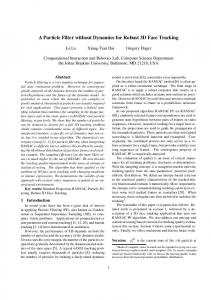
Flow¥lsyilzfltion
im&gs acajyliiiion tiigîipfiss îittêniig
IfflBije preprocasiBQ Dëtêcttefi mû ocs&on off
psnposs
i Estabftehiiêrttrf yyi
f
flflMyi: ! M-vi* t1yÉp|p
Camera orlenfalons
Dêtêfillilâi« of
Câïteiûft iali
Cifcyfatiort of now
partiel? positons TfiÄrti in object
tzz
e*:i l*#
»a»
Fig.
fields without
disturbing
the flow.
ft f
rpwtp
liUHr
5: PTV
fCintmalenioitf
flpjçaysj-
ffajsttOt t%ia
processing
scheme
Except the tracers, which
are
used the visualize the flow
can
be considered
as an intrusive component of the method, but with the right choice of particles leads to minimal and negligible disturbances (see in 4.1.). The particle motion is recorded by at
least two
synchronized cameras. In most PTV applications the cameras observe the flow from outside the object volume thus being located in a different optical medium than the particles. If the motion in a fluid is observed through a glass plate the optical ray passes through air, glass and fluid and is broken twice according to the refractive indices. If different media are involved in the optical setup then the optical geometry has to be modelled (see 3.3.). After
digitization the image sequence data is processed to segment the particle images and to extract their image coordinates. After the assignment of corresponding particle images from different views it is possible the determine the 3D particle position in object space by forward intersection. A tracking procedure reconstructs the particle trajectories. The existing PTV solutions either work with an image or object space based tracking algorithm. The new spatio-temporal matching algorithm, which was developed during the presented research work uses the information of image and object space for the tracking procedure simultaneously. The different PTV solutions are described in detail in chapter 5. an on- or
offline
15
2.2.
Techniques
for flow measurement
The
implementation at ETH uses a fully automated image processing procedure to extract the particle positions in image space (Maas, 1992b). As a first step a highpass filtering of the images to remove non-uniformities of the background intensity level is performed. After that, the particles are segmented by a thresholding algorithm. The image coordinates of the particles are determined by a greyvalue-weigthed centre of gravity. With the knowledge of camera orientation data determined in a system calibration it is possible the establish correspondences between the particle images. With at least two particle positions in image space the 3D position in object space is defined and can be calculated with a photogrammetrie algorithm. To get the 3D particle trajectories in object space a tracking procedure based on image and object space based information is applied. The results of PTV processing are three-dimensional velocity fields, which can be used for hydrodynamic analysis. A processing scheme of PTV is shown in Fig. 5.
Comparison
2.2.3.
Table 2 summarizes
of flow measurement
techniques
presented flow measurement techniques. Other overviews on the different methods are given in (Maas, 1992b) and (Virant, 1996). Compared to the measurement techniques obtaining pointwise information from one or a few probe locations, the temporal resolution of PTV can be considered as low. The major advan¬ tage of PTV is the simultaneous observation of a three-dimensional object volume, measuring not only all three components of the velocity vector but also providing trajectory information. Due to this fact PTV is the only technique, which offers the possibility to perform Lagrangian some
chararacteristics of the
measurements.
Concerning
the accuracy information shown in Table 2 the comparison of the potential of the hardly possible as the authors are using different measures to specify the
different methods is
quality of the results. For details about the potential of the different methods see (Jorgensen, 2002), (Heist/Castro, 1996), (Lai/He, 1989), (AIAA, 2003), (Bolinder, 1999), (Kompenhans et el, 1996) and (Maas et al, 1993). Commercial systems for CTA, PWA, LDA, L2F and PIV method
proposed
in this thesis is
mechanics and Water Resources
successfully Management
are
available
on
the market. The PTV
used for flow research at the Institute of
Table 2: Performance characteristics of the different flow measurement
Method
Spatial
Temporal
Dimension of
resolution
resolution
measurement
CTA
low
PWA
low
LDA
low
L2F
low
LIF
PIV
PTV
16
very
high
high very
high
1-3 1-3
high
1-3
very
high
very low
3
very
high
very low
2(3)
low
3
high
techniques
Results
Accuracy potential 1-3% of the ~
1-3
scale
Vectors
1% of the
Vectors
5% for
velocity scale, high turbulence
Vectors
signal
to
velocity
noise ratio
systematic random
5-10%
1% of mean flow
lateral 1:4000,
~
velocity
Vectors
Vectors
Vectors
depth 1:2000 Trajectories velocity vector
3.
3.
Photogrammetrie aspects
In this section the
Photogrammetrie aspects
for 3D PTV
for 3D PTV
photogrammetrie principles
used
by
3D Particle
Tracking Velocimetry are collinearity condition and its epipolar line intersection method to
described. First the fundamental mathematical model of the extensions build up
explained. A further section deals with the multi-camera correspondences in the case of a multi-media geometry. are
3.1. Mathematical model The
fundamental
matical
model
grammetrie
of
3D
mathe¬
photo¬ particle
coordinate determination is the
collinearity condition, that object states point, camera projective centre and image point lie on a straight line (Fig. 6). which
This mathematical formula¬
tion, which contains three coordinates
X0, Y0, Z0 of the projective center and three angles co, cp, k describing the direction of Fig. 6: Collinearity condition (camera model the optical axis, applies to a inverted for drawing purposes) pinhole camera model not regarding the influence of any distortions mainly introduced by the use of lenses. Considering the camera constant the principle point with its coordinates x^, y^ leads to the following equations:
X,
—
an
(X,-X0)
+
au
(Xl-X0)
+
(Xt
X0)
{X,-X0)
Xi,
(Y,-Y0)
+
a3l
(Z,-Z0)
a23-
(Yl-Y0)
+
a33
(Z,
+
a22
( y,
Y0)
+
a32
(Z,
+
a23-(Yl- Y0)
+
a33
(Z,-Z0)
a2l
•
-
c
and
Z0)
(4) fliz
y,
where
=
«is
•
-
are
image
coordinates of the
•
-
-
Z0)
position Xt, Yp Zp the up- are the elements of the 3x3 rotation matrix derived from the three angles co, cp, k. To meet the physical realities the model has to be extended by introducing the following parameters to
x'p y\
the
yh-c-
•
object point
at
the
compensate the distortion of the lens and electronic effects. These parameters within
a
calibration
procedure.
For
digital
close range
applications
a
very
are
common
determined
approach
to
17
3.2.
Handling
of the mathematical model
model the lens distortion is
k2, k3) and decentering following equations:
x;
x;
=
+
in
given
distortion
dx,
(Brown, 1971).
is modelled in
(pj, p2)
yl
=
yl
+
dy,
symmetric lens distortion (kj, polynomial approach given by the
The radial
with:
dx,
=
x\
(kxra
+
k2r'4
+
k3r'6)
+
px
(r'2
+
2x,'2)
dy,
=
y\
{kxra
+
k2rA
+
k3r'6)
+
p2
(r'2
+
2_y,'2)
,2
i
and:
r,
,2
x,
=
+
+
+
^
2p2x\yl'
'
2pxx\yl
,2
y,
In addition the influence of electronic effects from the
digitalization and storage, mainly the unknown difference of the clock rates of camera and framegrabber may have to be compen¬ sated. These effects can be modeled by applying an affin transformation (El-Hakim, 1986):
Due to linear
dependencies
x,
=
a0 +
axx\
+
a2y\
y,
=
b0
bxx\
+
b2y\
+
of the six parameters
(a0, b0,
bj,
aj,
a2, b2) of the affin transforma¬ of these parameters are intro¬
tion with the parameters of the
two
duced
scale factor a; in horizontal
as
collinearity equation only remaining parameters are the shearing angle a2.
unknowns. The two
coordinate direction and the
image
collinearity condition (4) in combination of the additional parameters (5), (6) leads to the following functional model, which is suited to be linearized as observation equations in a least squares adjustment: The
(x', y')
=
f(X0, Y0, Z0,
co, (p, k, c, xh, yh,
The 16 parameters
describing
transformation
introduced
are
ku k2, k3,
as
unknowns in
a
calibration
possible to apply the epipolar line intersection particle images from the different cameras.
3.2.
Handling
Spatial
procedure.
After their determina¬
method to establish
correspondences
of
of the mathematical model
The mathematical model •
(7)
X„ Y„ Z,)
the exterior and interior orientation, the lens distortion and affine
tion it is the
pu p2, au a2,
can
be used in three different modes:
resection: The parameters of the exterior orientation
X0, Y0, Zq,
co, cp,
k
and the
model c, xh, yh including the additional parameters are determined in the calibration procedure. In 7.4.2. the calibration of an image acquisition system used for 3D PTV is camera
described. •
Spatial intersection: After the correspondences 3D particle camera
•
18
Bundle
calibration of the system and the establishment of multi-view coordinates
can
be determined based
on
the orientation and
model parameters.
adjustment: Using multiple images of a scene, object point coordinates, camera orientation parameters
taken under different orientations, and
camera
model parameters
can
3.
Photogrammetrie aspects
for 3D PTV
be determined one
scale
simultaneously, based only on image space information and a minimum information in object space. This procedure has been used for the provision
reference values for the targets All three different modes
on
of
the calibration bodies.
used when
are
of
evaluating image
sequences with 3D PTV.
3.3. Multimedia geometry The motion of the
particles
is observed with
cameras
outside the flow
through
a
glass plate.
Therefore the rays have to pass through three different media, fluid, glass and air. Due to Snell's law the optical path is broken when refractive indices changes. Assuming homogeneity and
isotropy
effect
can
of the different
be modelled
optical media strictly (Fig. 7).
n3
Fig.
7: Radial shift for
(water)
and
considering
a
plane parallel glass plate
O(X0,Y0,Z0) N(X0,Y0,0) P (Xj, Yj, Zj) P (X,, Y„ Z.) PB (XB> YB> Zß)
projective center nadir point object point radially shifted object point break point
R
n1; n2, n3
radius in X/Y-plane refractive indices
ßi. ß2> ßs
angles
this
camera camera
in Snell's Law
X,Y-plane
compensation of multimedia geometry, taken from (Maas, 1996)
If the X-Y
plane of the coordinate system is chosen parallel with the plane interface glass/ water (or air/glass), some simplification are possible and only the radial shift Ai? has to be calculated to be able to use the collinearity condition equation (see in (Maas, 1996), p. 194). The radial shift is a function of the radial distance R of the object point P from the nadir point N of the camera, the thickness of the glass plate t, the depth ZP in the fluid and the refractive indices n, of the traversed media. Maas developed and implemented this approach for the PTV system at ETH (Maas, 1992b). In the PTV implementation for each camera discrete lookup tables with the radial shifts over the observed object volume are calculated and used to compensate the influence of the multimedia geometry. Further details about the multimedia geometry (also beside these exactly modeled aspects regarding the implementation in the PTV software are described in (Maas,
3.4.
Epipolar
line intersection
effects) 1992b).
and
technique
important approach used for the PTV method is the establishment of multi-image corre¬ spondences by constraints in the epipolar geometry developed by Maas. The epipolar geometry is used to establish the correspondences automatically. The powerful technique is successfully used for PTV (Maas, 1990), (Maas, 1991a) and (Maas, 1992b) as well as for other applications An
19
3.4.
Epipolar
line intersection
technique
(Maas, 1991b) and deformation measurement (Dold/Maas, 1994). This method requires the knowledge of the interior and relative orientation as well as the addi¬ tional parameters of the according images. Fig. 8 shows the epipolar geometry in a two camera arrangement. Using the coplanarity condition of the oriented image planes as
surface reconstruction
CM?2 (Ö^P' Ö^P') •
epipolar line in image space image the corresponding search the
x
=
(8)
0
Proceeding from an image point of the first area can be reduced to the epipolar line in the second image. In the strict mathematical formulation this line is straight, in the more general case with nonnegligible lens distortion or multimedia geometry the epipolar line will be a slightly bent line, which can be approximated by a polygon (Maas, 1991a).
Image
Fig.
In the
8:
can
be determined.
Image
1
2
Epipolar geometry in a two camera arrangement (left), example of intersecting epipolar line segments in a four camera arrangement (right)
by a certain tolerance e to epipolar bandshaped image space. The length / of the search area along the epipolar line can be restricted by the range of depth (Zmin, Zmax) in object space. The tolerance e to the epipolar line is strongly influenced by the quality of the calibration results. Due to the large number of particles ambiguities occur as often two or more particles will be found in the epipolar search area. The use of a third or a fourth camera allows the calculation of intersections of the epipolar line segments in image space, which reduces the search area to the intersection points with a certain tolerance. the
case
of real
experiment
data the search
line, which becomes to
a narrow
area
has to be extended window in
example of an epipolar line intersection in a four camera arrangement is shown in Fig. 9. Starting from the first view, the possible candidates for the marked point (58) are searched along the epipolar line l12 in the second image. For the candidates found in the second view
An
20
3.
the
Photogrammetrie aspects
for 3D PTV
123 are calculated and intersect with the epipolar line 113, which reduces the search area of possible candidates to the intersection point with a certain tolerance. Remaining ambiguities may be solved by analysing the fourth view. The epipolar line intersection is implemented with a combinatorics algorithm to establish unambiguous quadruplets, triplets and pairs of corresponding particle images (Maas, 1992b). epipolar
Although four
lines
the method
camera
is
be extended to any arbitrary number of cameras, the neither necessary nor practical.
can
usually
Camera 1
Fig.
9:
Principle of the epipolar line intersection
use
of more than
Camera 2
in
a
four
camera
arrangement
21
3.4.
22
Epipolar
line intersection
technique
4. Hardware components of
4. Hardware
3D PTV system
a
components of a 3D PTV system
In this section the technical
discussed. The
aspects for
is based
a
hardware setup and the
the
of
potential of the method are synchronous image sequences of a flow
technique recording neutrally buoyant particles. The hardware setup of a 3D PTV system consists of an image acquisition system with up to four cameras including a data storage device, an illumination facility and tracer particles to seed and visualize the flow. Whether high-grade components or off-the-shelf products come into operation is depending on the experiment requirements as well as on the available budget. The data acquisition system defines the achievable spatial and temporal resolution. on
visualized with small,
Because of the fast can
only give
an
developments of the different hardware components the following incomplete snapshot of the available products on the market.
sections
4.1. Visualization of the flow To enable measurements in
of the flow. In the
case
The
transparent medium such in liquids
of PTV
applications
the flow to be
or
gas
investigated
which should follow the motion of the fluid without
particles, important property tracer
a
is the
visibility
of the tracer
requires
a
visualization
is seeded with discrete
disturbing
it. A further
particles.
mainly influenced by the size and the density of the parti¬ density of the fluid and the particles should be kept small to avoid vertical drift velocity. In the case of flows in fluids this can be achieved quite easily, but it is hardly possible for flows in gases. In general slip and delay can be reduced by the use of smaller particles, which again decreases the visibility. flow-following properties
are
cles. The difference between the
Regarding the automated image coordinate measurement by using a grey value-weighted centre of gravity the particles have to cover at least 2x2 pixel in image space to be located with subpixel accuracy. But again the tracer particles must not appear too large in image space. If a high spatial resolution is requested the problem of overlapping particles has to be consid¬ ered. The number of overlapping particles grows linearly with the particle image size and approximately with the square of the number of particles per image. The size of the particles used in PTV applications is in the order of a few up to some hundred urn depending on the experiment. hydrogen/oxygen bubbles are used as tracers to visualize the flow, which can be produced by an aeration unit or electrolysis (e.g. in (Schimpfet al., 2002), where the investiga¬ tion of bubble columns is described). An experiment with two different kinds of particles is described in chapter 7.4. A selection of possible particles can be found in (Maas, 1992b), details about the light scattering properties are given in (Engelmann, 2000). In
some cases
23
4.2. Illumination
4.2. Illumination A decisive component of
mination •
Argon
a
Different
facility.
PTV setup with
light
a
sources can
strong influence
be
employed
for
on
a
the
image quality
is the illu¬
suitable illumination:
ionic lasers
Diode lasers
•
Halogen lamps
•
short
Halogen
•
lamps
diodes
Light
•
arc
The illumination
facility
should
provide a high and homogenous light intensity overall wavelength of the emitted light has to be appropriate to sensors used for the image sequence acquisition.
whole observation volume. The
spectral sensitivity
of the
light dangerous
provide
Laser
sources
the
monochromatic
deal with. Lasers
to
the
are
light with a high intensity, but are difficult or even expensive in comparison to the other mentioned light
sources.
Halogen lamps are easy to handle (e.g. very flexible in combination with fibre optics) and deliver homogenous illumination at very low costs. A disadvantage is the rather low light intensity with a strong blue component, which run contrary to the high spectral intensity of CCD sensors in the red wave band. Halogen short arc lamps show more or less the same prop¬ erties as halogen lamps but provide higher light intensity and their handling is more difficult. Diodes
easy to deal with and deliver
are
is the poor
homogeneous light
as
low costs. A
disadvantage
light intensity.
For the recent PTV
used
at very
experiments performed illumination facility.
at ETH a
continuous 20-Watt
Argon
Ion Laser
was
4.3. Sensors There is
great variety of image
the market, which could be
successfully applied image sequence acquisition for PTV purposes. Decisive properties are the geometrical temporal resolution. Further aspects are data storage as well as the costs. a
sensors on
for the and
In the
following some of these properties regarding their applicability for PTV. 4.3.1. Video
Reading video norms
norm
from
a
standard video CCD
that defines the
(Comité
RS 170,
a
are
described and discussed
(Charged Coupled Device)
timing and the level of the transmission. an interlacing technique):
Consultatif International des Radio
standard, which
used in USA. One The
devices
sensor
There
is
regulated by
are
two
a
different
related to
625 lines per frame. The vertical •
imaging
norm
(both strongly
CCIR
•
out
of
image
was
Communications) European reading (field) frequency is 50 Hz.
defined
by the
EIA
norm
with
(Electronics Industries Association) and is reading frequency is 59.9 Hz.
frame consists of 525 lines, vertical
by the video cameras can be recorded on analogue videotapes by a digitized off-line afterwards. The loss of quality caused by the inter¬ mediate storage of the image data on video tape can be avoided by on-line digitization with the use of framegrabbers. The resolution of the currently used data acquisition system for PTV is in the order of 640 x 480 and 768 x 576 pixels. analogue signal
delivered
video recorder and
24
4. Hardware components of
a
3D PTV system
Stroposcope #1 Digital Image
HDTV LD #1 III DD DE EHE BEBE
Processor 1
a ma turne
Nexus9000
D
DDD
i
i
21'HDTV
m
Monitor
^^^^^^^^^^^
Work Station DEC PWS600au
Fig.
4.3.2.
system with three High Definition TV cameras, laser disk recorders, digital image processor, taken from (Suzuki et al., 2000)
10: HDPTV
Image acquisition
with
High
Definition TV
cameras
system's image resolution is achieved by the use of high definition using High-definition CCD-cameras was built up at the University of the Tokyo at Department of Mechanical Engineering. As mentioned above, standard video cameras deliver images with 0.5 megapixels and less. High-definition CCD-cameras provide images around 2 megapixels. An existing system originally developed by Nishino et al. (Nishino et al., 1989) and later improved by Sata and Kasagi (Sata/Kasagi, 1992) consists of three Sony XCH-1125 TV cameras and three laser disk recorders (Sony HDL-5800). Their present image system provides image sequences with a resolution of 1920 x 1024 pixels (the system is described in (Suzuki et al., 1999)). A
possibility to
TV
cameras.
increase the
A 3D PTV
The 3D HDPTV system with its hardware components is shown in
Fig. 10. Stroboscopes synchronized signal employed Images captured by each recorded the laser disk recorder frames/s. The recorded images are then onto at 30 camera are A/D converted and transferred to a workstation. The higher resolution is thought to lead to a higher number of particle trajectories to be trackable in a velocity field. Compared to standard CCD cameras the costs for the high-definition system can be considered as rather high. According to Suzuki the costs for the system, which was built up in the year 1996, amount to 1 million US $. Some further remarks about this system, the data processing and its performance with the TV
can
are
for illumination.
be found in section 5.4.
25
4.3. Sensors
4.3.3. IEEE-1394
technology (Firewire)
The
high performance serial bus IEEE-1394, also called Firewire, offers a possible way for on¬ image sequence storage. The output of the camera is directly delivered in different image formats (greyscale, coloured, uncompressed and compressed). Due to the direct output no framegrabbers are needed. Normal VGA resolution (640 x 480 pixels) at a frame rate of 30 Hz can be captured in progressive scan mode. XGA (1024 x 768 pixels) and SXGA (1280 x 960 pixels) resolution is also available at smaller frame rates, which will increase soon considering the fast developments in imaging technology. Sychronization is possible by an external trigger. The given maximum bandwidth of is the limiting factor when temporal and geometrical reso¬ line
lution is concerned. IEEE-1394
4.3.4.
Integration
sensors were
not
modes
The conventional CCD
sensors
are
designed
for
video and TV. For these systems two alternative •
used for PTV at ETH yet.
in the
integration
integration mode uses the double integration resolution but high dynamic resolution.
•
field
use
of two
frame
interlacing scanning systems
modes
are
adjacent lines, giving
integration mode uses the integration of each odd line giving high vertical resolution but low dynamic resolution.
after
of
used:
integrating
low vertical
each
even
line,
Due to the time
delay between the acquisition of odd and even fields the image contents appears blurred if fast moving object are recorded. The best way to get rid of such interlacing effects is to use progressive scan cameras. Quite simply, progressive scan means that the picture information is accumulated simultaneously and the charges from all the pixels are transferred to one or two horizontal registers. The result is a non-interlace image with full vertical and horizontal resolution captured in a single rapid shutter event. Today's progressive scan cameras are available at reasonable costs and should be applied for image acquisition to provide good image quality at full frame resolution. Especially in the case of recording small moving objects the progressive scan readout can be regarded as the most suitable choice. Nevertheless a considerable problem has been identified by the image sequence acquisition with the progressive scan cameras JAI CV-M10 used in the experiments described in 7.3.3. At a recording rate of 60 Hz the signal from camera to frame grabber is transmitted through two different cables. As a negative effects this results in different signal magnitudes for even and odd lines. As no further experience with other types of progressive scan cameras were made, it is not possible to identify the mentioned effect as a general problem of the sensors of this architecture. PTV
4.3.5. Fill factor and The fill factor of
light sensitivity
photodetector and ranges in general form 20 % to 90 %. Because the sensitive area of a CCD sensor is only a fraction of its total area, on-chip lenses can be used to concentrate the light of the optical image into the sensor area of the pixel and thus increase sensitivity. a sensor
is the fraction of the
example
inactive
26
CCD
chips
back to the active
use
The
such
occupied by
the
microscopic lenses to redirect light from the areas pixels. Sony Hyper HAD® sensor structure has an on chip lens (OCL) located over each pixel. The Exwave HAD takes the Hyper HAD sensor tech¬ nology a step further (AudioVideoSupply, 2003). The OCL of the Exwave HAD CCD is a nearly gap-less structure, eliminating the ineffective areas between the microlenses. This enables the whole accumulated layer to receive the maximum amount of light. For
from SONY
sensor area
4. Hardware components of
4.3.6. Cameras with CMOS An alternative type of
sensors
besides CCD
cameras
CCD
common
(ROI) selective pixel rates. Available
readout
is offered
by
the CMOS
technology
In the recent years remarkable progress
(Complementary made in the development the
3D PTV system
technology
Metal Oxide
over
a
was Semiconductor). of this sensor technique. Some of the advantages of CMOS sensors sensors are blooming resistance, tuneable response, region of interest flexibility as well as low noise and low power consumption for high
(Silicon Imaging's MegaCamera) on the market provide full frame resolu¬ tion of 2048 x 1536 pixels at 30 Hz frame rate. Another camera, the Phantom v5.0 offers a maximum recording speed of 1000 pictures per second using the sensor's full 1024 x 1024 pixel array. Frame rates are continuously variable from 30 to 1000 pictures per second. An integral image memory is capable to record 4096 images in full format (for example 40 seconds at 100 Hz). Higher frame rates at reduced image sizes may also be selected using the Phantom
cameras
control software.
camera
The architecture of the the
chip, tions).
sensors
is flexible and allows
which could also increase the
arbitrary arrangement of the pixels on geometrical resolution (e.g. which staggered pixel posi¬ an
processing functions within the camera, such that the amount of data to be transferred to the system's memory or disk can be drastically reduced. Relevant operations like filtering, blob detection, centroid computations etc. could thus be performed on-board, leaving only pixel coordinates of the blob centers to be transferred. CMOS
cameras
allow the execution of
This may be useful for PTV applications as with the realtime-detection of the coordinates the storage of the image sequences could be avoided. However
particle image todays CMOS cameras are not yet capable to detect and extract the image coordinates of 1000 or more parti¬ cles at reasonable frame rates. Therefore and due to the significantly higher costs compared to CCD cameras no CMOS sensors were used for PTV applications at ETH yet. In consideration of the technical developments in the future CMOS sensors might be a valuable alternative to the currently used CCD cameras.
Synchronization
4.3.7.
To be able to determine the 3D cameras
at the
synchronization
same
of
a
position
of
a
time. Therefore the
multi-camera setup
can
moving particle it has to be imaged by at least two image acquisition has to be synchronized. The be realized in different ways.
quite simple method to get synchronized image sequences acquired by three monochrome cameras operating in combination with a single RGB-framegrabber. Each camera can be
A
treated as
as one
slaves. The
images, In the
tapes
a
which
case
of
of the three colour channels. One
image can
an
data of all three
cameras
be divided in monochrome
intermediate storage of
time code added to the
images
camera
is defined
is then stored in
images
as
one
master
and the two others
image
sequence of RGB
afterwards.
synchronized image sequences on analogue corresponding images.
video¬
enables to read
synchronization of four progressive scan cameras with two framegrabbers is described in (Stüer et al., 1999b) and (Stüer et al., 2000). In this setup the cameras are also synchronized by a master-and-slave mode to relieve the framegrabbers (Matrox genesis) from timing tasks, which were critical at high frame rates. One problem is to start the two framegrabbers simulta¬ neously. For this purpose, the two framegrabbers run in a trigger mode and need a TTL pulse that indicates when to grab the next image of the cameras. To provide a constant TTL pulse, a The
27
4.4.
System
calibration
synchronization unit was built that was connected to the v-sync of the cameras giving a TTL pulse at the chosen frame rate of the cameras. The operator can start TTL pulse and with it the two frame grabbers simultaneously begin to grab. The image data is stored in real time on hard disc via two RAID controllers (RAID stands for Redundant Array of Inexpensive or some¬ times "Independent" Disks). This procedure has the advantage that a degradation of the images is avoided and it facilitates a long measurement time. The system was tested for a measuring time of 2 minutes, but even longer measurement times should be possible. Only
when the motion of the
devices it
plexed 4.4.
might
be
system. This
System
An essential
particles is slow compared to the frame rate of the imaging sufficient if the images of the different cameras are acquired by a multi¬ was the case in the micro-gravity experiment described in chapter 7.4.
calibration
requirement
for
a
successful
the exterior orientation parameters
as
application
well
as
of the PTV method is the
matical model is described in section 3. The actual calibration
cameras
points,
which is
placed
into the
object
uses
a
of the mathe¬
reference
body with by all
imaged points on the
image the experiment
each
once
reference
be deter¬ describing mined. Depending on a suitable reference body has to be provided considering others the of the reference points, their visibility and coverage over the entire among accuracy observed object volume. As an example of such a reference body used for PTV see Fig. 52. For the different experiments, which were performed in the recent years several reference bodies of different sizes were produced at ETH. Details about the used reference bodies can be found in (Maas, 1992b), (Becker et al, 1995), (Stüer, 1999) and (Willneff/Maas, 2000).
body
coordinates the parameters
handling
volume and is
of the system. With the known 3D coordinates of the control
and the measured
of
the interior orientation parameters, lens distortion
and effects of the A/D conversion. The mentioned parameters and the known control
knowledge
camera can
4.5. Hardware of the 3D PTV system at ETH The system
currently used at the ETH Zurich was upgraded from offline to online image digiti¬ previous system, the image sequences were firstly recorded on analogue video¬ tapes and digitized afterwards, while in the new system two frame grabbers (Matrox Genesis) are used to provide online digitization and storage. The development of the hardware setup can be nicely traced comparing the systems described in (Maas, 1992b), Virant (Virant, 1996), Stüer (Stüer, 1999) and the most recently in (Lüthi, 2002). The length of the recorded digital image sequences is nowadays restricted by the storage device capabilities. The data rate for a 60 Hz full-frame camera with a resolution of 640 x 480 pixels is about 19 MB/sec, and hence in an experiment, which lasts for 1 minute four cameras deliver a total amount of about 4.5 GB image data. Some details about the recently used hardware setup and changes are given in section 7.3.3. A possible hardware design is shown in Fig. 11. zation. In the
28
4. Hardware components of
a
3D PTV system
channel cross-section
Fig.
11: Hardware
setup for channel
cross
section
experiments, adapted from (Maas, 1992b)
4.6. Potential of 3D PTV With
vectors
image
format of 768
of
more
than 1000
x
576
particles
pixels,
the method allows for the determination of
velocity using a four camera system. The relative accuracies of the vector components are approximately 1:4000 (standard deviation of X and Y coordinates over field of view); the accuracy of the depth component Z is typically by a factor of two to three worse than the components perpendicular to the main viewing direction. These figures are valid under controlled conditions; suboptimal illumination conditions, complex flows, temperature gradients or image noise may lead to a severe degradation of the potential. The length of the trajectories depends on the seeding density: With a lower number of particles in the observation volume the probability of 'loosing' particles due to unsolved ambiguities in the detection, the establishment of correspondences or in the tracking procedure decreases. In practice, particles could be tracked over several hundred frames when the number of particles in the observation volume was kept small (Virant, 1996). an
per time instant
29
4.6. Potential of 3D PTV
30
5. Overview
5. Overview
on
particle tracking
on
particle tracking
methods
methods
particle moving in 3D object space can be imaged as a 2D path in the image space of an observing camera. If corresponding particle images were found in at least two cameras the 3D particle position can be determined. If in addition the temporal assignment is possible, the trajectory can be reconstructed. Fig. 12 shows the trajectory of a particle in an object volume over four time steps and its according 2D paths in image space recorded with a two camera arrangement. The PTV system used at ETH works with up to four cameras to provide better spatial resolution. The goal of the tracking procedure is to select the correct link for the same particle from one time step to the next. A
Fig.
12: Particle
with
a
trajectory in image and object camera arrangement
space recorded
two
31
5.1. Coordinate based
spatio-temporal assignment
5.1. Coordinate based The
spatio-temporal assignment
object space based tracking technique for spatio-temporal matching corresponding particle positions in object space as well as in image space. The following criteria can be used for a reliable and effective assignment (Papantoniou/Maas, 1990):
uses
developed image
and
different criteria to find
•
The
•
The
•
In
velocity
of
a
particle
is limited in all three components of the motion vector.
Lagrangian acceleration of one particle) is limited. of
cases
probable
ambiguities
the
a
minimum and the maximum
space, but
a
particle (the
assignment
difference of two consecutive
with the smallest
Lagrangian
velocity vectors
acceleration is the most
one.
The first criterion defines
Lagrangian
of
three-dimensional search volume, whose size
velocity
acceleration defines
can
easily
a
on
the
in all three coordinate directions. The limitation of the
conic search
be transferred to
depends
image
area.
These criteria
are
formulated in
object
space.
From three consecutive time steps the difference of the
magnitude and direction of predicted of ambiguities a quality function is particle position used to get the final assignment as proposed in the third criteria. A particle and its possible link candidates in the following two time steps fulfilling the velocity and acceleration criteria are shown in Fig. 13. and found
can
be calculated. In the
case
tj+1
Fig.
5.2.
13: Particle motion and search volume in
Algorithmic aspects
for
tj+2
object
space, taken from
spatio-temporal matching
The two most
(Stüer
et
al., 1999a)
for 3D PTV
important processing steps of 3D PTV the establishment of spatial and of temporal correspondences between particle images in synchronous image sequences of multiple CCD cameras which were strictly separated in the existing implementations, have been unified (see in (Willneff/Grün, 2002) and (Willneff, 2002)). In former implementations the trajectories of the particles are reconstructed in two different ways: -
-
The
•
particle positions
are
determined for each
single
time step;
tracking
is
performed
afterwards in 3D space. In the previous implementation at ETH Zurich multi-camera correspondences are established by epipolar line intersection techniques in a first step,
trajectory reconstruction is performed in 3D space (see in (Malik et al., 1993) (Papantoniou/Maas, 1990) and (Papantoniou/Dracos, 1989)). A similar procedure is used by Kasagi and Nishino in the 3D PTV system of the University of Tokyo (see in (Kasagi/ Nishino, 1990), (Nishino et al, 1989) and (Nishino/Kasagi, 1989)). before the
32
5. Overview
•
Other methods first track the
on
particle tracking
methods
in
image space. Then the spatial correspondences between the 2D trajectories are established (e.g. (Engelmann, 2000), (Ge/Cha, 2000), (Guenzennec et al., 1994) and (Netzsch/Jähne, 1993)). particles
In the
following sections image space based and object space based tracking methods are examples of the according approaches are given. Based on the previous system at ETH a new spatio-temporal matching algorithm for 3D PTV was developed, implemented and tested. The principles of the method are described in section 6. described and
5.3.
Image
space based
tracking techniques
technique firstly tracks the particles in image space and thus provides the temporal matching leading to 2D tracks in image space of each camera separately. The spatial corre¬ spondences between the 2D tracks are established after that in a separate processing step to generate trajectories in object space. Fig. 14 shows the scheme of an image space based tracking method with its main processing steps. This
Image sequences of multi-camera setup, acquired by two CCD-cameras in a convergent arrangement often
Tracking of particles
in 2D
image approaches space (e.g. Fuzzy logic, neural networks) with
different
\ Stereoscopic correspondences problem, matching of the 2D tracks to generate particle trajectories in object space, requires system calibration and orientation
Fig.
14: Main
processing steps of
an
image
space based
tracking
method
operable system applying this tracking method is described in (Engelmann, 1998) and (Engelmann, 2000), where the image acquisition system consists of two CCD cameras. In his
A
33
5.3.
Image
space based
tracking techniques
Ph.D. thesis
(Engelmann, 2000) Engelmann gives a detailed view on the method and describes two different hardware setups, which were successfully used for the data acquisition for PTV. Two experiments were carried out at the circular Heidelberg wind-wave facility and at the newly constructed AEOLOTRON circular wind-wave facility. More details about the Heidel¬ berg wind-wave facilities can be found in (Hering, 1996) and (Schmundt et al., 1995). For the first
experiment a two camera setup equipped with Pulnix TM 6701 AN cameras was used to acquire image sequences with 60 Hz and a resolution of 648 x 484 pixels. In a second experiment two Sony XC-73CE (providing a resolution of 752 x 582 pixels) with a frame rate of 30 Hz recorded the hydrogen bubble velocimetry distribution. The temporal resolution was considered to be sufficient to determine the motion of the bubbles.
particle velocity and exposure time the particles appear as streaks. A first step to obtain the 2D trajectories in image space is a segmentation of the streak lines performed in each image. After the segmentation of the streak lines the temporal correspondence problem from one time step to next has to be solved. Wierzimok and Hering proposed a tracking method via interlaced images (Wierzimok/Hering, 1993). The integration time of the two fields of one image has a certain temporal overlap depending on the used camera and shutter mode. In the case of the Pulnix TM-640 the overlap was 50 % of the integration time. The temporal overlap is supposed to be a feature for the identification of objects in the consecutive images. Further details about this tracking approach via interlaced images can be found in (Hering, 1996). At low particle density a dilation operation is sufficient criterion for the correspondence match, but ambiguities will occur at a certain concentration. A set of Fuzzy variables was implemented to solve the ambiguities with a confidence measure (Hering, 1996). Five particle characteristic properties are taken as Fuzzy variables to determine a confidence measure for the solution of the temporal correspondence problem: Depending
on
the
•
The distance of the current streak from the streak in the
•
The distance from the current streak from its estimated
•
The difference of the current
•
The
•
The difference of the streak
grey-value
velocity
Fuzzy-logic lookup
tables
in the current
resulting
in
a
position
of the streak from the
difference of the streak in the current area
previous image
image
confidence
then link these five values. The candidate of the
image
velocity from the
from the
measure
largest
in the
previous image
previous
previous.
for each
confidence
possible correspondence
measure
is taken
as corre¬
sponding. A linear
or a
second order model is used for the
position
estimation of the streaks.
approach extended to three dimensions is applied in the actual PTV implementation at ETH (see in section 6.4.). The simple estimators are considered to be sufficient in most cases, nevertheless a more sophisticated estimator, which can be used is proposed in (Jahne, 1997) applying Kalman-filtering as a recursive linear optimal estimator. To reconstruct particle trajectories in object space the found temporal correspondences have to be matched in the stereoscopic views. Mainly three different constraints proved to be important for the stereo The
same
correlation: •
•
Temporal order, each trajectory consists of a list of subsequent, timely ordered streaks. For each streak a corresponding streak in the second image is required, otherwise the trajectory is split up in two or more trajectories. Ordering
Geometric constraint:
epipolar
34
constraint:
window of
a
Epipolar constraint, corresponding trajectories certain tolerance.
are
found within the
5. Overview
•
on
particle tracking
methods
Object property constraint: The relation of correlating to non-correlating streaks of two trajectories must not exceed a threshold. Two trajectories correspond to each other if the distance between the streaks varies only within the epipolar window
The
epipolar
constraint
ters of the two
camera
requires
a
calibration
procedure
system and is considered to be
to
one
determine the orientation parame¬
of the strongest constraints to solve
the
stereoscopic correspondences. Also for the PTV implementation at ETH the use of the epipolar geometry is a fundamental. The epipolar line intersection method (see in 3.4.) extended up to four cameras is very important for the solution of the multi-ocular correspon¬ dences in the PTV implementation at ETH. Again comparing the two implementations the multimedia geometry is strictly modeled in both approaches (see in 3.3.). Regarding the performance of the tracking method Engelmann does not provide according values in his thesis as later proposed in 7.1. applying neural networks for the tracking of particles is proposed in (Ge/Cha, 2000). stereoscopic particle tracking system consists of two non-interlaced Sony-8500 cameras with a resolution of 782 x 582 pixels for the observation of three-dimen¬ sional flow fields. Again tracking is performed in image space first. After the determination of the 2D particle positions in each frame their displacements are extracted in image space. To increase the spatial resolution they apply both Hopfield and stochastic neural networks for the tracking procedure. Based on a search of all possible tracks over four or five consecutive frames the potential tracks are extracted. A global energy value is then assigned to each valid track. As stated, neural networks are well suited to find the solution producing the lowest energy in an optimization problem. The extracted 2D tracks are stereoscopically matched to generate 3D tracks thereby representing the 3D velocity field. As a performance estimation the authors of (Ge/Cha, 2000) report that almost 600 particles could be tracked.
An alternative method
Their
A further PTV system
1994)
who tested
a
using image
system with
a
tracking is proposed in (Guenzennec et al., alignment for the acquisition of stereoscopic images.
space based
mirror
single camera, the mirror arrangement located in front of the camera lens leads to two different viewing directions for the left and right part of the image. The stereo angle can be varied by different arrangements of the mirrors. After a pre-processing of the images, the PTV algorithm determines the particle tracks from sequences of five frames in each of the two views using the concept of path coherence. Then a stereo matching tech¬ nique searches for stereo matched pairs of particle tracks in the two views. The system works with
5.4.
Object
one
space based
tracking techniques
correspondences in one instant of particle position first. The temporal matches are searched afterwards in the 3D object space. Fig. 15 shows the scheme of an object space based tracking method with its main processing steps.
An
object
space based
tracking technique
tries to solve the
time to determine the three-dimensional
The consequent
application of the method of intersection of epipolar lines allows the establish¬ ment of multi-image correspondences and the determination of 3D particle positions in object space (developed and implemented by Maas, see in (Maas, 1992b), briefly described in 3.4.). The obtained point cloud for every single time step serves as input data for the object space based tracking technique. The tracking procedure is described in more detail in (Papantoniou/ Dracos, 1989) and (Malik et al., 1993). Each n-tupel of images is treated without considering temporal coherences with previous or subsequent time steps. The list of 3D coordinates is the only information, which is used by the tracking algorithm. Remaining ambiguities, which cannot be solved by the epipolar line intersection method lead to missing 3D particle positions over one or more time steps. Despite the high potential of the method this is the main disadvan-
35
5.4.
Object
space based
tracking techniques
sequences of multi-camera setup, up to four cameras in the case of systems at ETH
Image
of
Establishment
particle correspondences with epipolar constraints and determi¬ nation of 3D particle positions, treating each single time step separately, requires system calibration. consequent
Particle one
Fig.
tage, causing
a
concerning just
15: Main
processing steps of
gap in the one
particle trajectory,
an
3D
use
of
Tracking performed in point cloud as input for
object
which
space based
probably
can
3D
object
each time
tracking
be closed
space,
step
method
by interpolation
if
time step.
operable system exists at ETH since many years and has been successfully used for various applications. A sample of publications about the projects of the recent years dealing with 3D PTV are (Becker et al, 1995), (Dupont et al, 1999), (Lüthi, 2002), (Maas et al, 1997), (Stüer, 1999) and (Virant, 1996).
An
A similar method
University of Tokyo at the Department of Mechanical Engineering. The 3D PTV system originally developed by Nishino and Kasagi (Nishino et al., 1989), (Nishino/Kasagi, 1989), Kasagi and Sata (Kasagi/Sata, 1992) and Sata and Kasagi (Sata/Kasagi, 1992) was used for studies in liquid flow measurements and was modified by Sata et al. (Sata et al., 1994) for airflow measurements. After the reconstruction of the particle positions of each time step the tracking is performed in object space. Sata and Kasagi evaluated the 3D particle tracking algorithm over multiple time steps by using a modelled Lagrangian
36
was
developed
at
the
5. Overview
on
particle tracking
methods
time spectra of velocity fluctuations. They also found that the size of the search region could be significantly reduced, if the turbulence characteristics time scale is sufficiently larger than the
imaging frequency. In 1993 Ninomiya and Kasagi (Ninomiya/Kasagi, 1993) showed that more than 600 velocity vectors could be obtained by tracking over four time steps using a standard NTSC
camera
setup.
recently used system is described in (Suzuki et al., 1999) and (Suzuki et al., 2000) consists of three high-definition CCD cameras. The hardware setup is briefly described in 4.3.2., the image acquisition system is shown in Fig. 10. Due to the significantly higher resolution of the imaging device Suzuki, Kenoya and Kasagi expected to obtain 6-7 times more particle trajec¬ tories compared to the former NTSC system. In a single-phase flow experiment an average of 1200 velocity vectors could be obtained, which is less than expected in advance. Compared to Virant (Virant, 1996), who yielded 1300 simultaneous velocity vectors from image sequences acquired with 512 x 512 pixels resolution, this number can be considered as rather low. In the arrangement used by Suzuki, Kenoya and Kasagi also particles outside the measurement volume were illuminated, so that the yield of velocity vectors is significantly decreased unlike the estimate owing to the increase of overlapping particle images. They claim to obtain more instantaneous velocity vectors when using semitransparent solid particles and only one single stroboscope to illuminate the measurement volume. The
algorithmic point neering at the University tracking method. From
an
of view the research group of the Department of Mechanical Engi¬ of Tokyo does not report of recent developments of the particle
37
5.4.
38
Object
space based
tracking techniques
6. 3D PTV based
6. 3D PTV based
Based
on
image
and
object
on
image
and
object
space information
space information
previous implementation at ETH a more consequent exploitation of the available thought to lead to improvements of the PTV method. In the previous imple¬ mentation at ETH Zurich the establishment of multi-camera correspondences is performed by epipolar line intersection technique treating each single time step separately ((Papantoniou/ Dracos, 1989), (Maas et al, 1993) and (Malik et al, 1993)). The tracking procedure is performed in object space exclusively using the 3D point cloud of each time step. A combined spatial and temporal assignment is supposed to lead to a higher tracking efficiency. on
the
information
6.1.
was
Spatio-temporal consistency
In the late
in multiocular
image
sequences
early nineties multiocular systems for the navigation of autonomous robots and vehicles were developed. At INRIA in France Ayache and Lustman developed a system with three cameras allowing the assignment of line segments from image triplets for each time instant of an image sequence (Ayache/Lustman, 1987). Navab and Zhang performed further developments at INRIA trying to combine the proposed stereo matching algorithm with a monocular line tracking approach (Navab/Zhang, 1992). Navab and Zhang realized that each of these processes may work faster and more reliably if they could borrow dynamically some information from each other. They proposed an unified iterative algorithm for both temporal tracking of stereo pairs of line segments and camera system ego-motion estimation. The dynamic cooperation between stereo matching and temporal matching processes was applied to image sequences acquired with a calibrated vision system, which was mounted on a mobile vehicle. The approach was found to be more reliable and less time consuming than using a classical stereo reconstruction for each single time step. eighties
and
spatio-temporal technique for checking the consistency of stereo range results and integrating them over time was presented in (Bolles/Woodfill 1993) and (Baker/ Bolles, 1994). The ultimate goal of this research was to develop passive range sensing technique that provide the spatial and depth resolutions required to detect small navigation obstacles. The experi¬ mental data was obtained by mounting a pair of cameras on a vehicle (HMMWV). The cameras were manually aligned with approximately parallel axes and recorded image sequences on VHS videotape as A
°c
r
|m
M,
\ DP Left Fig.
"^ J d
Right
Spatio-temporal "loop" check, taken from (Bolles/Woodfill 1993)
16:
the vehicle the
was
vehicle
driven
was
on
and off road. As
bouncing along over was not possible to
rocks and ditches it
39
6.1.
Spatio-temporal consistency
maintain
image
calibration. Therefore the
sequences
geometry, yet it could constrain the searches
matching algorithm
could
precise epipolar predicted line. The basic of the conventional stereo disparity epipolar approach system was to perform estimation in the two views ("left-right check") and optical flow estimation from present to past ("forward-backward check"). The stereo estimates are corroborated by performing a reverse right-to-left stereo match and verifying that the left-to-right result is its inverse. The optical flow estimates similarly validated by estimating the past-to-present flow. The principle of the spatio-temporal "loop" check is shown in Fig. 16. The two optical flow estimates Mj and Mr for each pixel in both cameras and the spatio-temporal transitivity of two stereo estimates from the current frame Dc and the past frame D„ can be checked to ensure that a four sided "loop" of matches is consistent. The spatio-temporal transitivity check is considered as consis¬ tent if the distance d between the matches Mr(Dc(P) and Dp(Mj(P) is within one pixel. a
precise
in multiocular
to a
rely
on
small number of lines relative to the
D'Apuzzo proposed a algorithm to track corresponding points from multiple views through image sequences and to compute their 3D trajectories (D'Apuzzo, 2002). The multi-image matching process is based on the adaptive least squares method (LSM) with additional geomet¬ rical constraints of the matched point to lie on the epipolar line (Grün, 1985). Both, the spatial correspondences between the images of the different views as well as the temporal correspon¬ dences between subsequent frames are computed using the LSM algorithm (Fig. 17). camera
1
camera
2
camera
3
time
i+1
Fig.
17: LSM
tracking: temporal and spatial correspondences established with LSM, taken from (D'Apuzzo, 2002)
The process starts matching corresponding points from the different views of the cameras. predicting the position in the next frame and the search of the position with the best
After
cross-correlation, the correspondence is established by least
matching (temporal LSM). position point linearly predicted previous time steps i-1 and i. The best value of cross-correlation between the image at time i and the image at time i+1 is found by scanning a search box around the predicted position. LSM is applied at that position and the result is considered to be the exact position of the tracked point in the new frame. This procedure is performed in parallel for the different images. To check the results, spatial LSM is computed at the positions resulting from the temporal LSM. If the differences between the two results do not exceed a certain threshold the point is tracked and the process continues to the next time step. The 3D coordinates of the tracked points for each time step are computed by forward intersection and its trajectory, velocity and acceleration is determined. The method can be used to track well-defined points on the human body. The
40
of the tracked
at
time i+1 is
squares
from the two
6. 3D PTV based
-,
on
image
and
object
space information
Image sequences of multi-camera setup, up to four cameras in the case of systems at ETH
Establishment of
particle with correspondences epipolar constraints and of
determination
particle addition
3D
positions, storage of
relevant
in
all
from
data
detection
particle process
Particle
Tracking
in 3D
point clouds, particle posi¬ 2D detections,
calculation of additional tion
from
unused in
more resulting completely longer reconstructed trajectories
Fig.
6.2.
18: Particle
tracking
based
on
image
Spatio-temporal matching algorithm
and
object
thus
space information
for 3D PTV
spatio-temporal matching algorithm uses the information extracted from image and object space simultaneously. The processing scheme of the tracking technique based on image and object space information is shown in Fig. 18. Compared to the previous system only the soft¬ ware solution is changed, the hardware requirements for the data acquisition remain the same. Our
ambiguities can be reduced drastically by the use of 3 or 4 cameras in a suitable configuration, they cannot be solved completely in case only one time step is consid¬ ered. Some detected particle locations still remain unmatched (obviously not all detections in image space can be matched, e.g. when a particle is visible only in one image). Assuming a 4camera setup a particle at best can be detected in four images, which delivers 5 redundant observations (4x2 image coordinate observations minus 3 object space coordinate unknowns).
Although
the number of
The number of image coordinate observations should therefore be sufficient for the determina¬ tion of the
according particle position
if
only
the
ambiguity
in the
correspondences
could be
41
6.2.
Spatio-temporal matching algorithm
for 3D PTV
Camera 4
Camera 3
J/
Epipolar constraints for spatial matches single time steps
in
Camera 1
Fig.
Camera 2
19: Redundant
spatio-temporal connections in the sychronized image courtesy by (Grün et al., 1996)
sequences of four cameras,
reliably. Along the epipolar line segments in the different views too many possible candidates are found especially when the particle density is high or/and the depth range of the object volume is rather large. solved
If
particle can be particle position in
prediction of the images this reduces the search space from an epipolar line segment to a single 2D search position with a certain added tolerance and can be determined by back-projection of the respective predicted particle position. Compared to the approach treating every time step separately this decreases the number of possible candidates causing less unresolvable ambiguities. a
tracked
over some
the next time step
consecutive time steps
can
be made. In the
a
case
quite
reliable
of two
-
-
possible matches in space and time, which can be used to recon¬ struct the motion of a particle recorded by four cameras. The different previous tracking approaches only use either the temporal or the spatial matching, while the enhanced method benefits from the use of both. Compared to the approach proposed in (Bolles/Woodfill 1993) and (Baker/Bolles, 1994) not only a pair of cameras (Fig. 16) is used for the image acquisition. Baker, Bolles and Woodfill performed a spatio-temporal "loop" check in image space to find consistent matches from stereo pairs. Fig.
19 shows the different
The
of
spatio-temporal consistency is also used for the enhanced PTV approach. initial tracks from particle positions established by applying the epipolar line method, the PTV approach predicts the particle position in 3D space for the next
principle Starting from
intersection
42
6. 3D PTV based
time step. As the search
positions
orientation data is available from
camera
can
be found
by back-projecting
the
on
a
image
and
object
space information
system calibration the according
predicted
3D coordinates into the
image
space of all views. The search in image space either leads to 3D particle positions or to formerly unmatched image particle detections, which can be used to calculate additional
particle positions. In contradiction to (Baker/Bolles, 1994) the spatio-temporal "loop" check is not performend in image but in object space. The consistency check of the particle motion could be extended from a simple geometrical model (as applied in the current PTV implemen¬ tation, see 6.4.) to a model also considering physical properties (Papantoniou/Dracos, 1989). The main issue of the
handling of redundant tracking information. Not only particle single time step but also the detections in image space are used to establish the temporal correspondences. In addition to the 3D point clouds used by the object space based tracking technique the new developed method handles also the image space based information. The redundant image coordinate observations combined with the prediction for the next particle position allow the establishment of spatio-temporal connections even when the velocity field has a high density or the movement of the tracer particles is fast. the 3D
After the
algorithm
new
is the
coordinates of the
the establishment of the
particle detection,
determination the data collection for the
correspondences and 3D particle position tracking algorithm can be divided in the following
steps: •
•
The
particle detection delivers a list of 2D image locations determined by a grey valueweighted center of gravity with subpixel accuracy including additional features like size and intensity of the according particle detection. The
application
detections at
one
of the
epipolar
line intersection method leads to
time instant. The
with the this •
according correspondence status of the processing.
The matched
particle
detections used in
number. Unused
particle
a
corresponding particle correspondence are labelled
detections remain unlabelled in
belonging to one correspondence are then used for the particle position in object space. The 3D coordinates are derived by a forward intersection. They are forming the initial 3D point cloud before the tracking is performed. particle
detections
calculation of the 3D
All this data is
the
previous implementation as well, but only the 3D point clouds tracking procedure. For the proposed approach the image and object space information is collected throughout the whole sequence and provides the input for the enhanced spatio-temporal matching algorithm for PTV. The tracking proce¬ dure using image and object space based information in combination with a kinematice motion modelling is described in 6.4. generated by
of each time step is used for the former
6.3. Alternative criteria for
temporal assignment
in
image
sequences
improve the assignment of particle images some characteristic attributes as size, shape and brightness might help to increase the reliability of the tracking procedure. But experience showed that these parameters depend less on the actual features of the particles itself as on the illumination conditions varying significantly for the different viewing directions of the observing cameras, (Racca/Dewey, 1988) and (Maas, 1992b). This leads to rather low correla¬ tion between the parameters of the particle image regarding one time step acquired with To
different
cameras.
assignment Within the
of
Due to this fact these parameters cannot further contribute to
a
reliable
corresponding particle images.
image
existent, which is
sequence of
one
supposed
allows
to
single an
it
be assumed that
higher improved assignment (Maas, 1992b). camera
can
correlations
are
43
6.3. Alternative criteria for
Trying can
•
•
to use
temporal assignment
the parameters of
in
image
particle image
a
sequences
as
additional criteria, the
following
methods
be considered:
area
based
matching
feature based
matching
The first method would try to match each
single particle image
with
a
certain
patch
size into
the
image space of the consecutive image. This method for the assignment seemed to be ineffi¬ cient for the search of corresponding particles. Applying area based matching of so-called
investigation light sheet is The
areas
in the PIV
technique (see
in section
2.2.2.4.)
is suitable because
only
a
thin
observed.
underlying
mathematical model of the
based
matching approach requires continuous, a three-dimensional object volume is objects. observed, therefore particles from different depth ranges and possibly contrary motion direc¬ tions or speed will affect an area based matching approach. A volume seeded with particles is a multi-layered object where occlusions of particle images are likely, which both makes an successful use of area based matching hardly applicable or even impossible. area
non-transparent and non-reflective
For PTV
In the context of the three-dimensional reconstruction of the exact use
image
features •
coordinates but also other features
these data, which is
already
available for
a
are
particle positions
determined. For this
feature based
matching.
reason
not
only
the
it is obvious to
The determined
particle
are:
the number of pixels
•
the dimension in
•
the
sum
x-
belonging
and
to a
y-direction
of grey values of all the
particle in
pixels
pixel belonging
to a
particle.
The
quality of the images has an influence on the parameters for the particle detection, which adjusted to reasonable values to detect as many particles as possible but avoiding mismatches. The images used for PTV show the particles as bright spots on a more or less dark background. The pixels belonging to a particle image are segmented with a simple threshold algorithm and the exact image coordinate is determined with a grey value-weighted center of gravity of segmented region. To avoid detection errors (e.g. caused by noise) a particle image has also to fulfil the properties such as a minimal and maximal size in x- and y-direction as well as a minimum sum of the grey values belonging to a particle. The choice of the threshold is made empirical, but is essential, because it influences directly all the mentioned particle features. With a higher threshold pixels, which belong to a particle image will be neglected and therefore do not contribute to the position determination nor to the features of the according particle. have to be
A former
investigation has shown higher correlation between corresponding particle parame¬ ters in consecutive images in sequences of single cameras compared to the images of different cameras (Maas, 1992b). Particularly the sum of the grey values seemed to be a suitable supporting feature, because of the lower influence of this parameter on the discretisation effects of the imaging system. Tests have shown that in spite of higher correlation between the sum of grey values of corresponding particles the contribution to an assignment is little. Insig¬ nificant differences of neighbouring particle images might be an explanation for that. Espe¬ cially particles, which are also close in object space will appear quite similar in image space because of their more or less same physical attributes and illumination conditions. Particles, which are close only in image space will probably appear different but can be excluded from the assignment because of their distance in object space.
44
6. 3D PTV based
A
has
typical particle image
a
size of 2
x
2 to 7
x
7
on
image
and
object
pixels. Especially
space information
for smaller targets in
motion the influence of discretisation effects is considerable. As size may change from 2 x 2 to 3 x 3 the assignment using the dimensions in x- and y will be rather obstructed or impossible than made
more
would occur,
reliable. Also with the
of
use
the
particularly considering
an area
mostly
based
rounded
matching problems of that kind particle images and reasonable
choice of matching parameters. The
epipolar
constraints in combination with
criteria for the
a
kinematic model
already gives
a
very strong
Therefore and due to the considerations about the
spatio-temporal assignment. an image sequence acquired by one camera, no significant improve¬ the ment was expected by use of the additional criteria mentioned above and thus is not imple¬ mented in the new spatio-temporal matching algorithm for 3D PTV. particle
attributes within
The used criteria for the
spatio-temporal assignment
are
the three-dimensional
particle posi¬
tions in one.
object space, the velocity and the acceleration from one time step to the consecutive This concept is similar to the approach proposed in (Papantoniou/Maas, 1990), except that
assumptions on the temporal assignment.
no
6.4.
correlation of
Tracking procedure using
Several
neighbouring particle
kinematic motion
motion
are
used for the
spatio-
modelling
employed for the kinematic modelling of the particle motion. A quite tracking applications is the time-dependent polynomial of order two (constant velocity) or three (constant acceleration). The latter leads to the following differential equation: approaches
can
be
familiar model for
3f(0 where
indicates the
x(t)
representing
=
position at time by a(t)
the acceleration x(t)
a(t)
=
const
v(t)
=
a(t0)- (t-t0)
x(t)
1 =
-a(t0)
(t -10)
(9)
0 t.
Through the integration of this equation velocity x(t)by u(t) one obtains:
and
and
(10) 2
+
v(t0)
(t
-
to)
+
x(t0)
where t0 is the
starting time of an object's path of movement. The model can be adapted to the alpha-beta-gamma model, which is proposed for tracking applications in (Fraser/Shao, 2001). This method requires the determination of the so-called tracking index leading to the gain coef¬ ficients a, ß and y for position, velocity and acceleration. Kaiman Filtering is also a suitable method for the filtering and prediction of moving objects, but requires a time-expensive computation of the covariance matrix for the filter gain coefficients (Hering, 1996). A reliable
extrapolation of a particle position with a more sophisticated model would require a positions from previous time steps. This is only the case if the particle was already tracked for some time steps, where the simpler prediction combined with a given search volume already succeeded to establish the links between the particle positions. Taking in account that particle positions might be noisy (especially in the viewing directions of the cameras, see in 4.6.) the use of a higher kinematic motion model would rather lead to disad¬ vantages than to an improvement. Considering the number of particles to be observed and resulting computational costs the implementation was kept simple and a second order predic¬ certain number of
tion is used.
45
6.4.
Due to the discrete
a
modelling
resolution of the
temporal
continuous formulation to •
kinematic motion
Tracking procedure using
discrete
one
image acquisition system
a
transition from the
is necessary:
particle position xp(t,) at time step tt a position xp(t1 x) for consecutive time predicted under the assumption of a piecewise constant particle velocity Ûpit,), eq. (11). A simple linear extrapolation is possible if the particle of step tt already has a valid link to the previous time step tt_\, otherwise the position from tt itself is used as search position. The temporal resolution At is given by the frame rate of the sensors used for the image sequence acquisition. Each particle is treated separately. From
a
3D
+
step ti+\ is
xp(tl l)
=
xp(t,)+Up(t,)-At
=
2-xJt,)-xJt,_i)
+
Xp\h)
ïïJt,)
with
(H) ~
%p\ti-l)
It
Assumptions on the correlation of neighbouring particle motion as proposed in (Papantoniou/Maas, 1990) are not used for the prediction of the particle position of the next time step. The
search
of suitable
backprojection
is
of the three-dimensional
all cameras, which are
candidates
be done when
easily
can
performed in image space. This requires the search position from object space to image space of camera
orientations and multimedia geometry
known.
performed in the image space of the cameras where the particle of step tt initially be found or matched (e.g. due to overlapping particle in one or more views). Based on a list of possible candidates a search position xp(t1 2) for time step ti+2 is predicted. If a valid link to the previous time step tt_i exists the predicted position Xp(tt 2) is calculated under the assumption of constant particle acceleration (model of second order, eq. (12)), otherwise again a linear extrapolation is used. The search is also could not
+
+
xp(tl 1) +
=
'
~
(5
with
For each found are
path
a
•
+
+
xp(tl i)
—
+
ap(tl
1)
Pyu
XJ
quality
At
up(tl 1)
+
=
+
+
xP(tl 2)
4
•
1 +
+
xp(tt)
Up\ti \)
—
+
=
ap(tl 1)
-
+
At
2
xp(tt_i))
C\l\
uP\ti)
~
At
criterion is calculated. The parameters for the
the acceleration and the direction
change
of the
particle, concerning
quality
measure
the time steps tb ti+1
and ti+2. The quality measure of a found path might be determined by an extended model that considers also the feature correlation of the particle image attributes (as size, shape and
brightness, described presented here. Conflicting particle If
in
6.3.),
connections
an
information, which is
are
avoided
by
the
quality
not
used in the
implementation
criteria.
from time step tt is already linked to the previous time step tt_i and connected to a particle of time step ti+\, but no candidate in step ti+2 is found, the
46
a
particle
can
be
quality
6. 3D PTV based
on
image
and
object
space information
factor is calculated from the time steps tt_\, tt and ti+\. In the tracking procedure the particle links are created between the time steps tt and ti+\. Therefore the 'last' particle position ti+\ of a
trajectory should also be connected with a link, but the position does not require information from time step ti+2•
•
If still
establishment to this last
particle
link could be established with the
already calculated 3D particle positions, remaining unmatched particle detections in image space from time step ti+\ around predicted location are used to determine an additional particle position (again reconstructed path has to fulfil the quality criterion). no
The
tracking possibility to
Fig.
can
be
extend
performed in progressive as well as regressive way. This offers a trajectory not only in forward but also in backward direction.
the the the
the
20 shows the
processing scheme of the tracking procedure. With this tracking procedure more complete trajectories is possible. Additional particle positions are formerly unused detections in image space.
the reconstruction of calculated from
Start
Particle
position at previous time step
Prediction of currant 3D soireft
position
Bacfcprejeeion of 3D search position in 2D imaae ipace Search for caniiiates in al vIbwb
LMofSDcitniiiafes
Preiictioii of 3D search
Baefcprojection
position for next time step
of 3D search
position in 2D imaga space
Search for caniiiates in al vIbwb
Search for nnmatchei parlcie tfatecdons in ai wmm
No
Yes
C9te«i»tionrf9*ioniii
particle positon
Reject Ink
Establish ItokfrOii previous to mmm
Fig.
20:
Processing
scheme of the
tracking procedure
47
6.5.
Exploitation
of redundant information for
ambiguity
reduction
tracking procedures the enhanced approach applied in only forward direction is called 'Enhanced (forward only)', applied in forward and backward direction it is called 'Enhanced (directional)'. The object space based tracking method, which tracks only the particles determined by the epipolar line intersection is called 'Previous'. To
distinguish
the different
Exploitation
6.5.
of redundant information for
ambiguity
reduction
The number of unsolved
ambiguities resulting from the epipolar line intersection technique can temporal context is considered. In the case of ambiguities particle trajecto¬ ries are often interrupted for only one or a few time steps. With the new algorithm these gaps can be bridged reliably and even the continuation of a trajectory is possible when the redundant information is exploited in a correct way. be decreased if the
Previous method
Enhanced method
Image
of
spaces
the different views
Image 4-3 0
ti-2 o
ti-1 9
^
t4+1
~
image space data used for tracking procedure !
No
9 9
°0
9
ti-1
^
4+1 .
4+2
O
ti-3
space
4-9
9
9
ti-1 9
ti-3 9
ti
9
.
4+3
Object 9
ti-1
Vi 9 4+1
4-2
.
4+2
9
'Zl
ti
ti-3
Tracking
\
result
ti-2
'Zl
N.
0
4+3
ti+i
4+2
0
.
ti-1
ti
ti+i
Vi
^\^ 4+2
/ti-3
Comparison of the use of available input data for the tracking procedure previous and the enhanced method.
derived with the
48
4+2
ti-1
4+3
:
.
ti-3
ti-1
/ti-3
21
result
ti-2 ti-1
Fig.
9
4+3
4+2
4+1
9 .
Tracking
ti-1
ti-2
9
ti-3
ti-3
9
Vi « 9
m
ti-1
space
*
9
4+2
-
ti
9
9
o
4-9 ©
*
1+ 0
w
9
Object
t.
9
4-2
ti-3
of
spaces
the different views
>v N.
4+3
\
and results
6. 3D PTV based
on
image
and
object
space information
Fig. 21 shows the differences in the use of object and image based information by the tracking algorithms. With the object space based tracking method (left) no particle position in time step tt can be calculated due to ambiguities in the epipolar line intersection. The available data used for the image/object space based tracking (shown right) are 3D particle positions (marked with filled circles) as well as image coordinates (unmatched particle detections are marked with unfilled circles). The result of the enhanced tracking algorithm closes gaps by additionally calculated particle positions from unmatched image coordinates. The goal of the enhanced algorithm is to yield longer trajectories. The length of trajectories can be increased by: •
•
•
•
Bridging a gap of a single time step by two fragments of a trajectory Bridging
a
gap of variable
Continuing particles
a
trajectory
an
additionally
between two
length
calculated
or more
particle position
fragments
of
in forward or/and backward direction with
A combination of the mentioned
a
to connect
trajectory
additionally
calculated
cases
Fragmented particle trajectories can be reconstructed more completely. With the enhanced method the existing gaps between the two or more trajectory fragments should be bridged and connected to one trajectory with increased length. This is possible by the knowledge of the motion from former time steps allowing a suitable extrapolation of the particle position and the use of yet unused image-space based information. Extrapolation is only used for prediction purposes. The calculation of the particle positions to close gaps is strictly based on image space observations (at least the 2D positions in image space from two different views). It is obvious that the influence of measurement errors is increasing when a particle position is calculated from fewer observations with a lower redundancy. But if the camera arrangement is suitable, the loss of quality is not substantial and still acceptable compared to an interruption of the particle trajectory. Considering •
•
•
the structure of tracking results the
The number of short The number of long The average
length
trajectories
of
•
The total
•
The total number of
length
trajectories
of all
following
be
expected:
will increase will increase
trajectories
will increase
trajectories
can
will decrease
trajectory
a
effects
will decrease due the connection of trajectory segments
These effects should be visible in
histograms showing the distribution of particle trajectories of specific lengths (or length classes). The qualitative change of the trajectory length distribution, which is expected for the PTV results is shown in Fig. 22. The distribution of the trajectory lengths yielded with the previous method reaches its maximum earlier than the enhanced approach, which corresponds to more and shorter trajectories. The distribution graph yielded with the enhanced approach is more flat and decreases slower with increasing trajectory length. As the total number of trajectories is expected to be decreased (due connecting of fragments to long trajectories) the integrated area under the enhanced graph might be of a smaller size. In the case of actual experiments the temporal resolution is limited by the frame rate of the image acquisition leading to a discrete distribution function of the trajectory length or specific length classes. The shape and relation of two distribution functions yielded with the different tracking algorithms will depend on the analysed data set, but should show up with the expected tenden¬ cies. A discussion about the yielded results of the reconstruction of more complete trajectories and some examples from simulated and real experiment data can be found in chapter 7.5. It has to be considered that all presented histograms are displayed in logarithmic scale.
49
6.6.
Non-algorithmic
limitations of
trajectory lengths
T CD O Ü
CD
CD
Trajectory length [1
with the
The
histogram of the expected trajectory length distribution yielded previous and enhanced PTV approach
Non-algorithmic goal
oo]
22: Qualitative
Fig.
6.6.
—»
limitations of trajectory
of the PTV method is to reconstruct
trajectories as long as possible. Besides performance implementation the motion of the particles itself can traceability of a particle. This is the case when a particle leaves the observation
the limitations of the reduce the
lengths
as
many
of the
volume.
ambiguities in the epipolar line intersection method as possible the object volume should be observed commonly by all available cameras. This is valid only for a certain percentage of the object volume. But even outside of the volume of full coverage particle trajectories can be reconstructed if the spatio-temporal connections can be solved. Based on the principles of the PTV method a particle moving in object space can only be tracked if it is in the field of view of at least two cameras. As the particle position is determined by forward intersection the 2D location in two image spaces is required. A particle moving from inside the observation volume to its border will sequentially disappear from the different field of view of the cameras until it will be completely vanished. To obtain
as
few
These conditions will that
from
particles intrude and leave particle trajectory.
end of the
50
change
experiment
the observed
experiment, volume during to
but in any case it can be assumed the sequence thus leading to the
6. 3D PTV based
6.7. Parameter
settings
for PTV
image
on
object
and
space information
processing
For the actual
processing of PTV data several parameters must be adjusted to yield reasonable setting of these parameters requires empirical knowledge as well as a-priori infor¬ about the flow field, which is under investigation.
results. The mation
The parameters •
•
•
•
•
Shape
concern
different aspects
as:
and size of the observation volume
Quality
of the calibration and orientation
Image quality Number of particles Motion of the
The
particles
roughly known by the experiment setup itself, but is also limited by the depth of focus of the cameras. Concerning the epipolar line intersec¬ tion technique (as described in 3.4.) a larger depth range of the observed object space leads to an increased number of ambiguities due to the longer epipolar segments to be examined. shape
and size of the observation volume is
The
quality of the calibration and orientation of the cameras has a strong impact on the processing steps. The direct influence on the accuracy of the three-dimensional particle coordinates determined by forward intersection is more or less obvious. But it also affects the establishment of the particle correspondences and thus contributes to the tracking different
results. An accurate calibration allows to a
smaller number of found
multi-ocular
use a
smaller tolerance to the
epipolar
line segments and thus
candidates have to be considered in the establishment of the
particle correspondences. This
results in
ities, which is beneficial for both the
previous
a
reduction of the number of
as
well
as
the enhanced
occurring ambigu¬ tracking approach.
An insufficient calibration makes less
impact on the number of linked particles determined with the enhanced method than with the previous approach. This can be explained as follows: The previous approach has to establish particle correspondences by the exclusive use of epipolar constraints, leading to more ambiguities the lower the calibration quality is. The enhanced method however considers the particle motion in object space, too. Compared to the previous method, it is therefore capable to resolve a larger number of ambiguities. In any case the calibration has to be carried out carefully as it is an absolute prerequisite for a successful 3D PTV application. The
by the illumination facility as well as the seeding parti¬ particle detection the image sequences should provide high contrast between background and particles. For the particle detection a threshold to segment the background is used. The image coordinates are determined with a grey value weighted center of gravity. image quality
is
mainly
influenced
cles to visualize the flow. For automated
For the
tracking procedure several parameters for the particle motion have to be adjusted. A particle motion the minimum and maximum velocity in all three coordinate directions is specified, the quality estimation of a particle link requires a value for the maximum valid acceleration and divergence angle. limitation for the
For the actual
application of 3D PTV a step by step advice thesis. Detailed background about the system calibration and be found in (Maas, 1992b).
is
given
in the
automated
appendix of particle detection
this can
51
6.7. Parameter
52
settings
for PTV
processing
7. Tests of the
7. Tests of the
The as
spatio-temporal matching algorithm
spatio-temporal matching algorithm
developed spatio-temporal matching algorithm for 3D PTV was tested with as with data from real experiments. Eight different data sets were used
well
mance
simulated data for the
perfor¬
tests.
All data sets
processed with the tracking approaches 'Previous', 'Enhanced (forward only)' (bidirectional)'. The tracking methods 'Previous', 'Enhanced (forward and 'Enhanced only)' (bidirectional)' were developed by the author and work as described in chapter 6. These approaches are based on object and image space based information. The method 'Previous' tracks only the particles, which 3D position could be determined by the epipolar line intersection. 'Enhanced (forward only)' and 'Enhanced (bidirectional)' are able to determine additional particle positions by using formerly unmatched particle detections. Performing the method in forward and backward direction yields most complete particle trajectories. were
and 'Enhanced
In addition two of the
eight data sets (see 7.3.3.7.and 7.3.3.8.) were also evaluated with the tracking 'TrackingHS', which was originally developed by Papantoniou, Dracos and Malik (Malik et al., 1993) and later modified by Stüer (Stüer, 1999). In comparison to the former approach Stüer's tracking approach does no longer support the principles of group velocities and minimum energy considerations as proposed in (Papantoniou/Dracos, 1989). For the two data sets, which were also processed with this method, the tracking rate was rather low and it was expected that better results might be yielded with the approach 'TrackingHS'. method
On the
one
hand the tests
are
performed
to compare
the other hand these tests should prove the tion
concerning
each
7.1. Definition of
the
operability
potential of the different methods, on developed software implementa¬
of the
single functionality.
performance
characteristics
To be able to evaluate the
performance of the PTV methods some performance characteristics are defined. As obvious performance characteristics can serve the number of particles p3D and the number of linked particles 13D per time step. To get rid off temporal variations within the image sequences a simple way to compare the performance of the previous and the enhanced method is the average number of established links over all time steps. The number of linked particles 13D is probably the most important value for performance evaluation concerning the
spatial
resolution.
But not
only
absolute values
number of established links method which is
can
13D
be used for the and
performance evaluation. The ratio between particles p3D gives the tracking efficiency eff3D of
the the
applied: eff3D
=
hi
(13)
53
7.2. Tests
using
simulated data
Due to the fact that the enhanced method has the
particle links l3D(add), the relative efficiency eff3D(rel) should also be related to the number of particles p3D(prev) derived with the previous method to achieve a better comparability: aff
(*0t\
-
hp(prev)
l3D(add)
+
capability
previous
method
was
used to
l3D(enh) >3D
quantify -
nA\
p3D(prev)
The ratio between the number of additional links the
additional
l3D(enh)
_
p3D(prev)
to create
the
l3D(prev)
established with
g3D of the enhanced method:
gain
l3D(prev)
and links
l3D(add)
l3D(add)
_
l3D(prev)
(15)
l3D(prev)
trajectories Ntm,- can be instructive however it is also decisive to consider the length ltraj of the trajectory as well. A trajectory of a particle might be in twice three interrupted resulting trajectory sections while an enhanced algorithm may be able to reconstruct just one complete trajectory without gap. Another possible way to assess tracking results is the average length avltraj of all the particles trajectories which could be reconstructed by the different approaches: The total number of all reconstructed
avi ltraj
Considering
(16)
traj
trajectories and their corresponding length of established links Ltm.- of all trajectories: =
J^traj
This total number of links
A
,y-
the total number of all
derive the total number
lished links
%h^
=
throughout
summary of the
aVltraJ
•
IV
traj
=
2^
Ltraj of all trajectories
it is
possible
to
traJ
can
also be calculated
as
the
sum
of all estab¬
the whole sequence.
performance given in
enhanced method will be
characteristics
for
comparison
the related sections where the
of the
previous processing of the
and the different
data sets is described and in section 7.5.4. The
in
different
also useful to compare the
analysis of the histograms (as described lengths or specific length classes is different approaches. 7.2. Tests The
input
using
6.5.) showing
data for 3D PTV
are
multi-ocular
synchronous image
sensors.
and
cameras.
To
perform
of the
a
first step
object
54
a
volume is
supplemented with specifi¬
describing
the interior and exterior
with simulated data it is also necessary to simulate realistic hardware design including the specifications
a
image acquisition system.
7.2.1. Generation of simulated In
sequences
tests
less reasonable flow field and
configuration
of
results of the
These additional informations consist of
cations from the hardware components and parameters
a more or
tracking
trajectories
simulated data
additional information to model the
orientation of the
the distribution of
image
sequences
three-dimensional flow field with
generated.
For each
single
a
time step
random a
set
particle
distribution in
of three-dimensional
a
chosen
particle
coor-
7. Tests of the
dinates is created, which then cameras.
To model the
sensors
can
be
reprojected
to
the
commercial standard video
spatio-temporal matching algorithm
image planes cameras are
Without
corresponding
assumed.
restrictions
the
to
the assumed lenses
validity ered
of the
as
general consid¬
are
distortionfree and the
size is set to 640 of 10
pixelsize
x
x
480
10
image with
pixels
urn
.
a
The focal
distance is chosen to 11.0 mm, which leads in combination with
object image of
distance of 200
an
mm
average to
good
coverage. The considered values
the
different
according
parameters
are
existing operable 3D PTV hardware designs and today's camera techniques. The parameters of the exte¬ to
rior orientation that the
camera
chosen in that way configuration leads to
are
well-defined intersections of the
Fig.
rays and
23: Simulated camera
configuration showing a four setup and the observed object
typically
volume with vortex flow
are
similar to
a
used for 3D PTV. The
uration is shown in
Fig.
optical
hardware setup
config¬
23.
principal point is assumed to be in the see section 3.1.). Additional parameters image sensor (for sensor modelling the distortion of the lens or electronic effects (shearing 5, scale in sx) are not used. As mentioned above this can be done without restrictions to the general validity and not using those parameters just simplifies the generation of the simulated image data. The images are generated by reprojection of the 3D particle coordinate to 2D image space. After the choice of some describing features like size and brightness the synthetic image is modified that the parti¬ cles appear as bright spots on a dark noiseless background. To define the interior orientation of the exact center
cameras
of the
the
model
resulting image sequence data is processed with the 3D PTV software in the same way as the data acquired during real experiments. The data generated for the simulation tests can be varied in manifold ways regarding the camera setup, the number and motion of particles as well as the length of the sequence. The reconstructed particle trajectories can then be compared with the initially defined velocity field, which is known unlike real experiments. The tracking results were investigated regarding the completeness of the reconstructed trajectories, not concerning the accuracy of the reconstructed particle positions. The
7.2.2. Simulation of
a
vortex flow field
To test the
performance of the developed algorithm a vortex flow field is simulated. The parti¬ circularly around a common axis parallel to the z-direction of the object coordinate system. In addition the particles move along this axis, the z-component of the motion vector is a random value out of a given interval and changes individually for each particle during the progression of the sequence. The vortex flow field is shown in Fig. 24. The visualization shows a selection of the reconstructed trajectories resulting from the PTV processing, not the simu¬ lated reference trajectories. cles
move
55
7.2. Tests
using
Fig.
simulated data
24: Vortex flow
be tracked
The size of
particle
a
field, showing a selection (ca. 200) of the particles, which could the complete sequence of 51 frames
over
particle image
but remains the
is set to 3
same
the
simplify performed only
x
3
pixel.
The
in each view of the
sum
of grey values is individual for each
cameras
and is
kept
constant
during
the
of the sequences the backprojection of the image coordi¬ pixel accuracy, which leads to some deviations between
generation integer the simulated and reconstructed 3D positions. Depending on the simulated motion and seeding density particles can leave the object volume or overlap each other in image space. Even when four cameras are used not all ambiguities in the correspondences can be solved by the geometric constraints of the epipolar line. Therefore not all particle positions can be recon¬ structed per time step not to mention be tracked over the time. A particle image of the simu¬ lated vortex flow is shown in Fig. 25. sequence. To
nates
56
is
with
7. Tests of the
Fig.
25: Particle
image of
simulated vortex flow
(left),
spatio-temporal matching algorithm
detail view
(right)
overlapping particle images not all less than 1350 particles per image can be detected image space. Therefore and due to ambiguities in the epipolar line intersection method even less particles can be reconstructed in object space. From the 1500 simulated particles around 1250 per time step can be reconstructed in 3D. An important parameter for the performance of the tracking method is the number of linked particles but also the number of blunders. The number of linked particles can be specified easily, unlike the number of mismatches. Setting the tracking parameters empirically the acceptable movements of a particle are defined. The analysis of the results concerning wrong tracks can only be qualitative. Using a suitable 3Dviewer helps to review the reconstructed particle trajectories. Due to
-
-
in
~
1400 en
100
--
CT
o
CD t
11
O •*—>
O
11
CD
"ÖT
10
1
-H "I
--
•*—>
i
o
Bl
l_
CD
11
.a
E 3
z
+
I
I
I
CO
CN
I
i
m
O)
CM
CD
i
00
i
Bl
Bl
(N
O
CN
CN
H
I
L-rm L-rM
i
CO
CN
4
i
Bl
i I
OS
CO
CO
CO
CO
^1-
OO
CM
CD
o
CN
CO
CO
-
1
11 11
1
II
^1-
i
ïn OO
Trajectory length [frames] Fig.
Histogram of the trajectory lengths obtained with previous and enhanced approach applied to the data set 'simulated vortex'
27:
7.3. Tests
using
PTV
real data
applied in real experiments, the method's capability has to be tested with respective performance of the method is influenced by many factors as the image quality, seeding density, particle velocity conditions in the flow, calibration and more. With just simulated data sets a thorough testing is not possible. For this reason various data sets from As PTV should be
data sets. The
59
7.3. Tests
using
real data
experiments were investigated in processing of the MASER 8 data set, which different
this
section.
addition in
chapter 7.4. the was acquired under micro-gravity conditions is described in detail. The data sets differ in many aspects as particle density, flow field character and hardware setup thus providing a good basis to prove the applicability of the developed method. For two of the experiments only a limited number of image data was available for the tests, but anyway could contribute to the performance evaluation of the tracking method. In
7.3.1. Data set 'Trinocular' This data set
investigation of open channel flows. A three camera setup was used to record the flow field of this experiment. The cameras were mounted in a stereoscopic arrangement with their axes intersecting at about 50 degrees. A 3 Watt argon-ion laser was used to illuminate observation oflOx lOx 1.5 cm. The cameras and the illumination facility were mounted on a carriage system driven by a stepper motor running along the channel. Further details about the experiment can be found in (Papantoniou/Dracos, 1990) and (Papantoniou/Maas, 1990), a description of the water channel is given in (Bertschler, 1985). was
obtained at the 24
m
open channel flume of the ETH for the
acquired with the first PTV hardware setup at ETH; nevertheless it is suitable performance of the tracking methods. The images acquired by Aqua-TV HR480 cameras with 1/2" frame transfer integration. Since video disks or image sequence memory were not available the video data was intermediately stored on three analogue video recorders and were digitized afterwards to a resolution of512x512 pixels at a frame rate of 25 Hz. The data set
to test
was
the
To be
able to read
corresponding images videotapes, a synthetic binary pattern, which codes a sequential image number, is added to the video signal of all three cameras. Despite the intermediate storage causing deterioration of the signal the quality of the image sequence was high. The from
the
number of time steps used for the tests 31. The ment
the
camera
arrangement for this experi¬
is shown in
cameras
are
was
Fig. 28,
the
optical convergent forming
axes a
of
tetra¬
hedron, which leads to well-defined intersec¬ tions of the accuracy
epipolar lines. The calibration quite high, nevertheless the
were
epipolar intersection led to a certain number of ambiguities, which might partly have been solved by a four camera setup. Making use of the spatio-temporal context these ambiguities could be solved even when only three 28: with three cameras cameras are used for the image acquisition. Configuration Fig. The reconstructed velocity field is shown in Fig. 29. As shown in Fig. 30 the number of links was increased by almost 40 % while at the same time the number of unlinked particles was reduced. In other words, regarding this data set it was possible to establish more links with the enhanced method than 3D particle positions with the previous approach. The increased
trajectories.
60
tracking efficiency also has a strong influence on the length of the reconstructed trajectory length avltra, could be increased by factor 2 (see Table 4).
The average
~
7. Tests of the
Fig.
29:
Velocity field 'Trinocular', showing
As the available
all
trajectories
spatio-temporal matching algorithm
tracked
longer
than 4 frames
experiment is limited to 31 frames both tracking approaches could track a certain number of the particle throughout the complete sequence. The previous method was able to track 82 particles over the entire sequence while with the enhanced method 204 complete trajectories were obtained. The number of trajectories longer image
sequence of this
than 15 frames could be increased from 294 to 590.
61
7.3. Tests
using
real data
Table 4: Performance characteristics
Tracking
N1raj, avl1raj
trap uvHraj
Number of trajectories
method
and
L1raj
-'traj
of the data set 'Trinocular'
Total number of all
"traj
Average trajectory length avl^j
2'240
7.7
17'243
1'569
13.4
20'949
1'567
14.3
22'391
established links
Ltra.-
Previous
Enhanced
(forward only) Enhanced
(bidirectional)
800 ,r.
7nn
t;
Rnn
«
^nn
-n
-
BJBSBJ
^^SBBS B^BB^Bj
4UU
B^S^BB B^BjB^Bj SBB^BI
?nn
B^BjBBH
-
Q. *
p
?nn
z
i nn
B^BjB^Bj
-
B^BjB^Bj B^BjB^Bj B^BjB^B] BBBBBB
n
Previous
Fig.
BBBBBB
Enhanced
Enhanced
(forward only)
(bidirectional)
D Unlinked
114
69
64
Linked
474
632
682
Average number of particles and links over 31 time steps determined with the previous and enhanced PTV approach applied to the data set Trinocular'
30:
The
frequency distribution of the trajectories (Fig. 31) shows that the enhanced approach is significantly superior in the reconstruction of longer trajectories (longer than 12 time steps) compared the previous method. Except of the already explained gathering effect due to limited sequence length the characteristic of the frequency distribution is in good coherence to the expected improvements (as mentioned in 6.5.) and the results of the evaluation of the simulated data set described in section 7.2.2.
62
7. Tests of the
spatio-temporal matching algorithm
1000
Previous D Enhanced
0 co ü o
100
E CO CT
o
CD
S
io
o
CD
CD .a
E 3
00
Trajectory length [frames] Fig.
Histogram of the trajectory lengths obtained with previous and enhanced approach applied to the data set Trinocular'
31:
7.3.2. Data set 'Forward In the framework of
acquired
at ETH.
facing step'
'Investigations of separation on a forward facing step' Stüer performed the research work (Stüer, 1999). As the data
7.3.1. the measurement
PTV
data sets set
were
described in
conducted in the open water channel, for details about the
experi¬ (Virant, 1996) and (Bertschler, 1985). A regulated radial pump pumps water in a closed circuit and the throughput is controlled by a magneto-inductive flow-meter. The cross section of the test area was 560 mm x 80 mm and the entry length was long enough to get a fully developed laminar parabolic flow field in the observation area. The height of the step was 20 mm over the whole span. This gave a channel height to step height aspect ratio of 4:1. The flow field was still laminar with an unsteady recirculation zone in front and on the step. The observation volume was 80 mm x 100 mm x 30 mm and placed at a fixed position in the middle of the channel and on top of the forward facing step. Particles enter and leave the obser¬ vation volume and for this reason it is obvious that particle cannot be tracked for infinite time. ment
facility
was
see
63
7.3. Tests
using
real data
The flow to be
investigated
with flow markers with -
63
urn.
a
was
seeded
diameter of 40
The observation volume is illu¬
minated
by two 400-Watt halogen-shortarc lamps, which have a high output effi¬ ciency of polychromatic light. The
motion of the flow markers
are
continu¬
ously recorded by four CCD cameras (RS 170, Jai CV-M10, progressive scan) with a spatial resolution of 640 x 480 pixels and a temporal resolution of 30 Hz. The chipsize of these CCD cameras is 1/2". The cameras are synchronized by a master and slave setup and oper¬ ating in shutter mode so that the short exposure time avoids a streaky imaging of the moving particles. The
Fig.
images of the four cameras are digi¬ tized and losslessly compressed by two frame-grabbers (Matrox Genesis) and
32: Four
camera arrangement used for observation of flow separation at a forward facing step
stored in real-time
on
hard disc via two
procedure has the advantage that the degradation of the it is minimized and facilitates a long measurement time (the reliability of the system images was tested for a measuring time of 2 minutes, even longer measurement times should be possible). The four- camera arrangement of this experiment is shown in Fig. 32. The distribu¬ tion of the particles of the flow was quite inhomogeneous and the seeding density can be considered as rather high, additionally some disturbances occurred due to scratches and stains on the bottom of the channel leading to some mismatches in the establishment of correspon¬ dences. The reconstructed velocity field is shown in Fig. 33. The forward facing step itself is not included in this visualization. The number of particles was around 1400; the number of established links was more then 800 with the previous method reaching more then 1000 links with the enhanced method. The results concerning the number of particles and links are shown in Fig. 34. RAID
Table 5: Performance characteristics
Tracking
method
Ntraj, avltraj
'trap u,vltraj
Number of trajectories
and
Ltrai
traj
controllers. This
of the data set 'forward
facing step
Total number of all
"traj
Average trajectory length avltraj
1915
5.2
9'971
1818
6.2
11'316
1814
6.6
11'975
established links
Previous
Enhanced
(forward only) Enhanced
(bidirectional)
64
Ltra.-
7. Tests of the
spatio-temporal matching algorithm
Ë
y
Fig.
33:
Velocity field forward facing step, showing
1400 en ^-
54: Front view of the
Fig.
7.4.3.
camera
—
—"
arrangement
Image preprocessing
In the framework of this
project
two
image acquisition campaigns
were
performed.
The
purpose of the first campaign (parabolic flights, described in section 7.4.4.) was to test the JET module under similar conditions as to be expected during the second one, the actual experi¬ ment
of the MASER 8
processed with
PTV
a
flight (see
certain effort
data. The steps of preparation
are
in section
7.4.5.). Before the image sequences could be of image preprocessing was necessary to get suitable input
described in this section.
While the data of the
parabolic flight campaign was quite satisfying, the quality of the MASER 8 flight images was significantly lower. The data was recorded in two ways during the MASER 8 flight. But not only the ground tape data has a high noise level, also the flight tape data shows less quality than the test images acquired during the parabolic flights carried out in 1998 (Swedish Space Corporation, 1998). This preprocessing contained the following steps and was applied to the data sets of both campaigns: •
Creation of
background image for each of the four cameras to remove nonground intensity level due to reflections and the intensity profile of the illumination. The first images are recorded before the particle injection and contain no particle images. For each view an images with no particles served as background image. To reduce the effect of adding high frequency noise from the background image to the sequence a
suitable
uniformities of the back
84
7. Tests of the
image were •
In the
were
resulting images was
the
The
filtered with
a
low pass filter. The
background images
then
image.
particles
as
appear
stains
bright
on
a
dark
background.
Each
added to itself to increase contrast.
To get rid of the defocussed
each •
images
subtracted from each sequence
image •
these four
spatio-temporal matching algorithm
camera) images
was
regions
used to cut out the
recorded
by
on
the
regions
the left CCD had
handle this the contrast in this
edges
images
was
a
of the sequence
images
a
mask
(one
per
of interest.
higher
noise level than the other
cameras.
reduced to decrease the number of false
To
particle
detections, which otherwise would disturb the establishment of particle correspondences. After the
image preprocessing the particles appear as bright spots on a more or less dark back¬ ground as generally required for 3D PTV. An example of the image preprocessing is shown in Fig. 55. Another advantage is that for all four cameras the same parameters for the particle detection can be used because the differences in the illumination are homogenized to a common level. The difference between the grey values of the imaged particles and the back¬ ground is 10 up to 100. After this preprocessing the image sequence data could be used for PTV evaluation.
Original
Image
(cut
sequence
image
Sequence image after preprocessing
mask
out defocussed
Fig.
55:
Background image (for subtraction from original)
edges) Image preprocessing of
sequence
images
85
7.4.
Application
of 3D PTV in space 'MASER 8
7.4.4. Parabolic
Project'
flight campaign
To prove the
applicability of the system the JET module was tested during the 29 ESA para¬ flight campaign (Swedish Space Corporation, 1998). To achieve similar conditions as during the MASER 8 campaign the test experiments were conducted under micro-gravity condition achieved by parabolic flight path. During three parabolic flights with an Airbus A300 in total 10 image sequences were acquired. The image sequences were processed with PTV to derive trajectories of the moving particles. As described in (Willneff, 1999a) all of the acquired sequences were processed successfully. In some of the experiments only a rather low number of particles were released into the observation volume by the particle injection unit. In this section only the processing and the results of one representative data set is discussed.
bolic
7.4.4.1.
Processing
of
parabolic flight
data
example of the parabolic flight data sets the image sequence 'pb08' over 70 time steps (equivalent to 14 s) is analysed. Due to a low number of particles moving with moderate veloc¬ ities the tracking of the particles should be possible without exhausting the potential of the PTV method. The reconstructed velocity field of the 'pb08' data sets is shown in Fig. 56.
As
an
Fig.
86
56: Velocity field of parabolic flight sequence 'pb08', showing tories which could be tracked longer than 30 frames
only
the
trajec¬
7. Tests of the
Fig.
spatio-temporal matching algorithm
Average number of particles and links over 70 time steps determined with the previous and enhanced PTV approach applied to the data set 'pb08'
57:
previous and the enhanced tracking method. Also in the case of this data sets the enhanced method yielded a significantly higher number of particle links than the previous approach. The average length avltraj of the trajectories was increased by almost factor 3. The longest trajectory obtained by the previous method has a length of 60 frames. Namely this could only be elongated to a length of 66 frames with the enhanced method, but at the same time the trajectories longer than 60 frames was increased to a number of 34. Fig. 58 shows the distribution of the trajectory lengths, which again shows good coherence to the expected effects described in 6.5. Fig.
57 shows the average number of
particles
and links
by applying
the
~
The
yielded results of the parabolic flights are quite promising, proving technique for space applications like the planned MASER 8 campaign. Table 10: Performance characteristics
Tracking
method
A^ra/-, avltraj
Number of trajectories
and
Ltraj
the
applicability
of the data set
of the
'ph08'
Total number of all
"traj
Average trajectory length avltraj
1'206
1A
8'924
627
18.1
11'331
562
21.9
12'345
established links
Ltraj
Previous
Enhanced
(forward only) Enhanced
(bidirectional)
87
7.4.
Application
of 3D PTV in space 'MASER 8
Project'
1000
_çd co ü to ü
CO CT
O to
CD O -i—
measure, middle> 539.00 Match: Point
2.00
372,
=>
zoom
corresp areas,
right> show epipolarline
micron, RMS
0.010/0.010/0.030
0
sigmaO
=
5.25
==
Fig.
67: Main window of PTV software
The
JnlxJ Change
Main Parameters
Change Calibration Change Tracking Fig.
106
mm
positioning (l.sq.)
68: Submenu
Parameters
Parameters
Change
Parameters
settings for the PTV processing can be through three different parameter windows (to be opened under the submenu Change Parameters, shown in Fig. 68). The windows for the editing of the parame¬ ters can be found under Change Main Parameters (shown in Fig. 69), Change Calibration Parameters (Fig. 70) and Change Tracking Parameters (Fig. 75). edited
Appendix
=
iBlxj
Main Parameters Number of
cameras:
(4
Name of 1.
image: inngAineMai25Carn1.111
Calibration data for 1
camera
ICarnl
Name of 2.
image: inng/meMai25Carn2.111
Calibration data for 2.
camera.
(Cann2
Name of 3.
imago: img/meMai25Carn3.111
Calibration data for 3.
camera.
lCam3
Name of 4.
image: inng/meMai25Carn4.111
Calibration data for 4
camera1
|Carn4
F Highpass-Filter
F
P Frame
TIFF-Header
C Field odd
C Field
even
Refractive indices: ^
j___
^^
|__
Parameters for
max
npix:
Sum of grey value:
(4
[TOOCT (100
3 I ring:
Img: [22
J2
npix in
x:
(30
max
discontinuity: (30
Size of
First:
images.
Basename for!
min
min for
Last:
img/meMai25Cam2. img/meMai25Carn3.
Basename for 4. sequence:
|img/meMai25Carn4.
Zmin:
-80
Zmaa:
-50.0
Xmax:
25.0
Zmin:
-80
Zmax:
-50.0
for ratio
nx:
(0
correspondences min
02
corr
for ratio ny.
02
0.02
epipolar band [mm):
(0.02
sum
Tolerance to
(0
of gv:
npix: (0.02
weighted correlation: (10
12
crosses:
layer data
-5.0
for ratio
(30
113
Xmin.
corr
y:
inngAineMai25Carn1
sequence:
Basename for 3. sequence:
corr
npix in
processing
Basename for 2 sequence:
Criteria for
Img |15
mm np« in j>;
100
Illuminated
min
4.
k.
Parameters for sequence Sequence
p
min npix in max
Tolerable
JgTkT
thickness of glass [mm):
particle recognition
2.
Greyvalue threshold, 1.lmg:|8 min npix;
p738
m^&:
M Fig.
A.4 Data
69: Main
parameter window
Input
The
processing of image data with PTV requires for each camera a valid video sequence stored in TIFF- (8 Bits/Sample, single image plane) or as raw data files. The respective flag for TIFF or raw file must be set. The filename for the sequence image is a combination of a basename indicating the camera and a current number. For each camera an orientation data file (name.ori) and an additional parameters file (name.addpar) must exist and has to be accessible for PTV.
107
Appendix
=
Calibration Parameter! Camera 1, Calibration
image:
JCarnl
Orientation data:
(Caml.ori
Camera 2, Calibration
image:
(Cam2
Orientation data:
(Cam2.ori
Camera 3, Calibration
image: (Cam3
Orientation data:
(Cam3.oii
Camera A, Calibration
(Cam4
Orientation data"
(Cam4
image-
File of Cooidinates
F
P Frame
TIFF-Header
horizontal:
(0
01
Target recognition
min max
p0
1.:
Qreyvalue threshold,
npix:
Sumofgreiivalue:
pOOO pOO
(0
npix in
x:
(7
max
npix in
x:
(50
Tolerable discontinuity:
(1
Image 1
PI:
|masfl2
pi;p
lmage3
1=^.
P2:|5
even
01
pu
4.: min
npix in