A Spherical Cap Preserving Parameterization for ... - Jonathan Dupuy

A Spherical Cap Preserving Parameterization for Spherical Distributions JONATHAN DUPUY, ERIC HEITZ, and LAURENT BELCOUR, Unity Technologies Real-time: analytic spherical-cap integration

Offline: joint BRDF/spherical-cap sampling Joint MIS (ours)

64spp MIS (previous)

64spp Fig. 1. Real-time application (left). We approximate BRDFs with our distributions and shade with sphere lights in real-time using their analytic spherical-cap integral. The scene is rendered at 1080p and runs at 60fps on an NVIDIA 980 GTX. Offline application (right). We compute the reference image with the exact BRDFs using importance sampling techniques. We use our distribution as a proxy for the BRDF and generate better samples that are distributed jointly inside the lights and close to the BRDFs. This joint sampling scheme is unbiased and has lower variance than multiple importance sampling with separate BRDF and light sampling. We introduce a novel parameterization for spherical distributions that is based on a point located inside the sphere, which we call a pivot. The pivot serves as the center of a straight-line projection that maps solid angles onto the opposite side of the sphere. By transforming spherical distributions in this way, we derive novel parametric spherical distributions that can be evaluated and importance-sampled from the original distributions using simple, closedform expressions. Moreover, we prove that if the original distribution can be sampled and/or integrated over a spherical cap, then so can the transformed distribution. We exploit the properties of our parameterization to derive efficient spherical lighting techniques for both real-time and offline rendering. Our techniques are robust, fast, easy to implement, and achieve quality that is superior to previous work. CCS Concepts: • Computing methodologies → Reflectance modeling; Additional Key Words and Phrases: spherical distributions, integration, sampling ACM Reference format: Jonathan Dupuy, Eric Heitz, and Laurent Belcour. 2017. A Spherical Cap Preserving Parameterization for Spherical Distributions. ACM Trans. Graph. 36, 4, Article 139 (July 2017), 12 pages. DOI: http://dx.doi.org/10.1145/3072959.3073694

1

INTRODUCTION

Spherical integration problems arise in many different areas of computer graphics. Because the current set of mathematical tools possessing closed-form solutions under spherical integrals is currently limited, solving such problems remains a computationally intensive task. In this paper, we focus on the problem of integrating spherical © 2017 ACM. This is the author’s version of the work. It is posted here for your personal use. Not for redistribution. The definitive Version of Record was published in ACM Transactions on Graphics, https://doi.org/http://dx.doi.org/10.1145/3072959.3073694.

distributions over spherical caps. Such integrals arise when spheres are used in rendering techniques, typically in the case of sphere lighting. A sphere light is a light source of spherical shape. Traditionally, such light models have been approximated by infinitesimal point and/or directional lights, depending on their location in 3D scenes. While infinitesimal light sources are much cheaper to simulate than sphere lights, they tend to produce unrealistic behaviors: since they do not have an area, they cannot be directly observed nor reflected by specular surfaces. For this reason, the offline rendering industry has started to discourage their use in favor of area lights (see for instance Pixar’s Renderman documentation [2016]), and we expect the point and directional lighting models to be respectively replaced by sphere and spherical-cap light sources in the near future. The real-time rendering community is also engaging in this transition, but at a much slower pace. This is due to the lack of sufficiently fast and robust solutions to the problem of integrating spherical distributions over spherical caps, as acknowledged by game-engine developers [Karis 2013; Lagarde and De Rousiers 2014]. In order to overcome this problem, we introduce a novel family of spherical distributions that have specific analytic properties for spherical caps, which we call Spherical Pivot Transformed Distributions (SPTDs). We obtained the properties of SPTDs by looking for transformations that have an invariance property over spheres, and found the family of 4D Möbius transformations. Our theoretical contributions are: • In Section 3, we identify a restricted set of 4D Möbius transformations that map the 3D unit sphere onto itself. We provide an intuitive 3D geometric interpretation for this subset of transformations and show that it preserves spherical caps. ACM Transactions on Graphics, Vol. 36, No. 4, Article 139. Publication date: July 2017.

139:2 •

Jonathan Dupuy, Eric Heitz, and Laurent Belcour

• In Section 4, we show how to use the Jacobian of this transformation to create novel parametric spherical distributions that have specific properties for spherical caps, such as integration and sampling. We believe that SPTDs provide useful mathematical properties that have been missing from the rendering toolbox. Indeed, besides determining the solid angle covered by two intersecting cones [Oat and Sander 2007], it currently seems that there are no parametric distributions for which the integral over a spherical cap can be computed practically. SPTDs offer a new way of solving this problem and bring new possibilities for rendering. To support this idea, we demonstrate the benefits they bring to important rendering problems: • In Section 5, we leverage the analytic integration of SPTDs against spherical caps to improve the quality of real-time sphere-light shading; Figure 1 (left) shows a real-time rendering of a complex scene illuminated by sphere lights that relies on our technique. • In Section 6, we leverage the sampling properties of SPTDs against spherical caps to improve the convergence of Monte Carlo sphere-lighting techniques; Figure 1 (right) compares the convergence of an importance sampling technique we introduce against a state-of-the-art multiple importance sampling technique.

2

RELATED WORK

Spherical Distributions. Several spherical distributions have been used for rendering purposes, such as von Mises-Fisher lobes [Fisher 1953] or Anisotropic Spherical Gaussians [Xu et al. 2013]. Unfortunately, none of these distributions can be analytically integrated over spherical caps. Actually, we have found only two distributions with analytic solutions to spherical cap integrals, namely the uniform distribution and the clamped-cosine lobe [Snyder 1996]. Note that solutions exist for Phong lobes [Snyder 1996], but they are expressed in terms of power series, which makes them impractical to compute and importance sample. Due to this very limited set, some authors have looked into basis functions such as spherical harmonics [Kautz et al. 2002], but these approaches are limited to low frequency behaviors. In contrast, our distributions can have arbitrary frequencies and be integrated against spherical caps with exact analytic forms. Real-Time Sphere-Light Shading. Sphere lights have been desired for a long time in the field of real-time rendering. Since no analytic solutions are known in the general case, some authors employ ad hoc techniques such as the most representative point [Drobot 2014]. Unfortunately, such approaches can result in visual artifacts [Lagarde and De Rousiers 2014]. Another solution could consist of tessellating the sphere into polygons and rely on a polygonal-light shading technique [Arvo 1995; Heitz et al. 2016; Lecocq et al. 2016]. However, the complexity of such techniques scales at least proportionally to the number of edges produced by the tessellation, leading to unreasonable computation times. In order to avoid this limitation, Lecocq et al. [2016] propose an ad hoc technique to mimic the effects of sphere lighting using a single polygon, but admit it exhibits artifacts. In contrast, our real-time sphere-lighting technique is robust and of reasonable computational cost. ACM Transactions on Graphics, Vol. 36, No. 4, Article 139. Publication date: July 2017.

Material-Light Joint Sampling. Importance sampling the product distribution (or joint distribution) of the scattering distribution and the light is a longstanding problem in graphics. However, we are not aware of a practical formulation of the joint distribution, even in specific cases such as ours. Indeed, existing work focuses on the joint sampling of BRDFs and environment lights through basis projections [Clarberg et al. 2005], hierarchical data structures [Cline and Egbert 2006; Rousselle et al. 2008], or dense rejection sampling [Burke et al. 2005]. We restrict ourselves to spherical lights but provide a lightweight and practical method to generate samples for both surface shading and volumetric integration. Linearly Transformed Spherical Distributions. Heitz et al. [2016] recently introduced a family of parametric distributions that have closed-form solutions under spherical polygon integrals. They derive their distributions by exploiting the Jacobian of a transformation with an invariance property with respect to spherical polygons. Our approach is similar to theirs in the sense that we also exploit the Jacobian of a transformation with an invariance property. For this reason, we chose to follow the layout of their exposition in Section 4.

3

GEOMETRY OF THE PIVOT TRANSFORMATION

In this section, we introduce the sphere-invariant transformation that we exploit to parameterize our spherical distributions. Since our transformation is a special case of the quaternionic Möbius transformation, we start by providing a self-contained mathematical background on quaternions and Möbius transformations in Section 3.1. We then focus on the derivation and properties of our transformation in Section 3.2 and prove that it is invariant with respect to spherical caps in Section 3.3.

3.1

Quaternionic Möbius Transformations

Definition. A Möbius transformation—also called linear fractional transformation or bilinear transformation—is mostly known as a circle-preserving, bijective map for complex numbers; it is practical for describing geometric transformations of the 2D plane with compact algebraic expressions [Yaglom 2014]. In this paper, we consider a generalization of the complex Möbius transformation to the space of quaternions, i.e., 4D space. A quaternion is a 4D vector q = (wq , rq ), wq ∈ R, rq ∈ R3 , to which is assigned a noncommutative multiplication rule p ? q, an inner product p · q, and a ¯ respectively defined as [Hanson 2006] conjugation rule q, p ? q = (wp wq − rp · rq ,wp rq + wq rp + rp × rq ), p · q = wp wq + rp · rq (⇒ q · q = wq2 + |rq | 2 ), q¯ = (wq , −rq ) (⇒ q ? q¯ = (q · q, 0)). A quaternionic Möbius transformation д is then any transformation of the form д(q; a,b,c,d ) = (a ? q + b) ? (c ? q + d ) −1 ,

(1)

where q,a,b,c,d are quaternions, and q −1 = q¯ ? ((q · q) −1 , 0). Equation (1) combines several 4D transformations, including translations, uniform scalings, rotations, reflections, and spherical inversions [Hertrich-Jeromin 2003]; the displacement are controlled by the quaternion parameters a,b,c and d.

A Spherical Cap Preserving Parameterization for Spherical Distributions • 139:3

S ω

C

C

S2

ωc

ψc

rp

д(ω ) д(C ) д(S) (1)

(2)

(3)

(4)

Fig. 2. Geometric properties of our pivot transformation. (1) We define a pivot transformation as a straight-line projection through a 3D point rp that maps any point ω located on the unit sphere S 2 onto another point д(ω ), also located on S 2 . Our pivot transformation is also spherical- and spherical-cap invariant: it transforms (2) spheres into spheres and (3) spherical caps into spherical caps. In this paper, we parameterize a spherical cap C with (4) a direction ω c ∈ S 2 and an aperture angle ψc ∈ (0, π ].

C

ωc

ω1 ω2

S2 rp

д(ω 1 ) ψc0

ω 0c

ω 0c

д(C ) д(ω 2 ) (1)

(2)

(3)

(4)

Fig. 3. Determining the properties of a spherical cap after performing a pivot transformation (the red cap is transformed into the green cap). (1) We work on the plane (drawn in gray) that intersects the red and green cap direction vectors ω c and ω 0c , and the pivot point rp . (2) This plane intersects the boundary of the red cap at two points ω 1 and ω 2 . (3) We project these points through the pivot point rp to retrieve two new points д(ω 1 ) and д(ω 2 ), which lie at the boundary of the new cap. (4) We determine the parameters ω 0c and ψc0 of the transformed cap from these two points.

Sphere-Invariance Property. Quaternionic Möbius transformations are bijective mappings that preserve spheres1 [Hertrich-Jeromin 2003; Wilker 1993]. Intuitively, this means that a quaternionic Möbius transformation maps any set of points located on the surface of a (4D) hypersphere embedded in 4D space onto the surface of another hypersphere, also embedded in the same 4D space. This property also holds for spheres of lower dimensions embedded in 4D space, i.e., (3D) spheres and (2D) circles. This is the key property that we leverage to derive novel spherical distributions that can be integrated and importance sampled analytically against arbitrary spherical caps.

3.2

Pivot Transformations

Mathematical Definition. We specialize the quaternionic Möbius transformation in order to create a transformation that maps S 2 , the unit 3D sphere located at the origin, onto itself. Mathematically, our transformation translates into constraints for the parameters ¯ and of Equation (1): we effectively set a = (1, 0), b = (0, rp ), c = b, 1 Möbius

transformations also map restricted sets of spheres to planes. Since we do not have to deal with such sets in this work, we assume here, without loss of generality, that spheres are preserved under Möbius transformations.

d = (−1, 0). By expanding Equation (1) with our parameter constraints, we can express the transformation occurring within the 3D subset of quaternionic 4D space with 3D vector algebra: д(r; rp ) =

(r · rp − 1)(r − rp ) − (r − rp ) × (r × rp ) (r · rp − 1) 2 + |r × rp | 2

.

(2)

Note that since this transformation is a special case of the quaternionic Möbius transformation, it is defined for—and effectively affects—any point located in 4D space. Intuitive Definition. Our transformation has an intuitive interpretation on the sphere S 2 , which is shown in Figure 2 (1): it consists of mapping the points at the surface of the sphere onto its opposite side with respect to a 3D point rp ∈ R3 located inside the sphere. Hence, we refer to this class of transformation as a pivot transformation, parameterized by a 3D pivot point rp located inside the sphere S 2 , i.e., |rp | < 1. Double Composition. Our geometric interpretation for the pivot transformation makes it clear that our transformation cancels on the sphere S 2 when applied twice. This property also holds for any ACM Transactions on Graphics, Vol. 36, No. 4, Article 139. Publication date: July 2017.

139:4 •

Jonathan Dupuy, Eric Heitz, and Laurent Belcour

other point in 3D space: r = д(д(r)) ⇒ д

i.e., −1

= д ◦ д.

ω c0 =

(3)

Sphere-Invariance Property. Since the quaternionic Möbius transformation preserves spheres, our mapping does too as we derived it as a special case; Figure 2 shows how our pivot transformation affects a sphere different from S 2 but located in the same 3D space. While the location and scale of S 2 remains unaffected after applying a pivot transformation, the same observation cannot be made for other spheres. This is because the pivot interpretation we propose only holds for S 2 , which is sufficient for deriving our spherical distributions (Section 4). Jacobian. The Jacobian of the pivot transformation restricted to the sphere S 2 defines the parameterization of our spherical distributions presented in Section 4. As we show in Appendix A, the expression of this Jacobian for any direction ω ∈ S 2 is

д(ω 1 ) + д(ω 2 ) . |д(ω 1 ) + д(ω 2 )|

(6)

In addition, we determine the aperture angleψc0 of the pivot-transformed spherical cap д(C ) with a dot product ψc0 = cos−1 (ω c0 · д(ω 1 )) = cos−1 (ω c0 · д(ω 2 )).

4

(7)

SPHERICAL PIVOT TRANSFORMED DISTRIBUTIONS

In this section, we introduce Spherical Pivot Transformed Distributions (SPTDs), a new set of spherical distributions with specific analytic properties over spherical caps. A SPTD is a variant of an input spherical distribution whose direction vectors have undergone a pivot transformation. We define the new distributions obtained in this way, and discuss their properties.

2

∂д(ω) * 1 − |rp | 2 + . = 2 ∂ω , |ω − rp | -

(4)

Figure 2 (3) shows the deformation produced by the pivot transformation at the surface of S 2 .

3.3

Pivot Spherical-Cap Invariance

Spherical Caps. We define a spherical cap on S 2 as the portion of S 2 that is cut off by a right cone whose apex is located at the origin of 3D space; Figure 2 (4) shows the geometry of this parameterization. Under this interpretation, any spherical cap C ⊆ S 2 is described by the two parameters of the right cone, namely its direction ω c ∈ S 2 and aperture angle ψc ∈ (0,π ]. Note that the solid angle Ac ∈ (0, 4π ] of a spherical cap is Ac = 2π (1 − cosψc ).

(5)

Invariance Property. We prove that spherical caps are preserved under the pivot transformation in two steps. First, we know that, by construction of the pivot transformation, the intersection between S 2 and the cone that parameterizes the spherical cap maps to S 2 . Second, we know that the pivot transformation—because it is a Möbius transformation—maps circles to circles. Hence, a spherical cap, whose boundary is a circle on S 2 , is mapped onto another spherical cap, whose boundary is another circle on S 2 . Parameter Determination. Figure 3 (4) shows the three points (drawn in green) that we compute to determine the parameters of a pivot transformed cap. We denote д(C ) ⊆ S 2 the spherical cap obtained after applying a pivot transformation to an input spherical cap C . Let ω c ,ω c0 ∈ S 2 respectively denote the direction of C and д(C ). We observe that the points rp , ω c and ω c0 always lie on the same plane; Figure 3 (1) illustrates this property. The input cap’s boundary intersects this plane at two points, which we denote by ω 1 and ω 2 ; Figure 3 (2) illustrates this property. We project these two points through the pivot and onto the opposite side of S 2 , obtaining two new points д(ω 1 ) and д(ω 2 ); Figure 3 (3) illustrates this operation. Then, the direction of the new cap д(C ) is oriented towards the mean direction between the two points д(ω 1 ) and д(ω 2 ), ACM Transactions on Graphics, Vol. 36, No. 4, Article 139. Publication date: July 2017.

D std

SPTD Variants

Fig. 6. Examples of SPTDs. The top and bottom SPTDs are created for various pivot points from a uniform and clamped-cosine spherical distribution, respectively.

4.1

Definition

Original Distribution. We use D std to denote the original input distribution that we wish to parameterize with a pivot. The shape of D std drives the shape of the transformed distribution; Figure 6 illustrates a few pivot transformed variants of a set of simple spherical distributions. Pivot Transformation. We create a new distribution D by applying the pivot transformation that we introduced in Section 3, i.e., by applying Equation (2) to the directions that constitute the original distribution. The pivot can be seen as a concentration parameter of intensity |rp | towards the direction of rp ; Figure 6 illustrates this effect. Note that we can recover the original distribution via the double composition property of the pivot transformation, i.e., ω i = д(д(ω i )). Closed-Form Expression. The magnitude of a SPTD is the magnitude of the original distribution D std towards the original direction

A Spherical Cap Preserving Parameterization for Spherical Distributions • 139:5 ω i ∼ D std

pdf[D std ]

(1)

(2)

(3)

ω i 7→ д(ω i )

(4)

pdf[D]

Fig. 4. Geometric construction of a SPTD. Given (1) an input spherical distribution associated with (2) a set of direction vectors, we create a pivot transformed distribution by (3) applying our pivot transformation to the set of direction vectors of the original distribution, resulting in (4) a novel distribution with specific analytic properties over spherical caps.

д(C )

C (1)

(2)

(3)

(4)

Fig. 5. Integrating and sampling a SPTD over a spherical cap. (1) Integrating a SPTD D over a spherical cap C is equivalent to (2) integrating the original distribution D std over the spherical cap д(C ). It follows that if we can (3) importance sample D std over a spherical cap д(C ), then we can also (4) importance sample D over the spherical cap C by applying the pivot transformation to the samples from D.

ω i weighted by the change of solid angle measure due to the distortion produced by the pivot. Using Equation (4), we obtain ∂ω i def D(ω) = D std (ω i ) ∂ω ∂д(ω) = D std (д(ω)) ∂ω 1 − |rp | 2

C

д(C )

(10)

Figure 5 (1, 2) provides a geometric interpretation of this result. 2

+ . = D std (д(ω)) * 2 , |ω − rp | -

(8)

Hence, if D std has an analytic expression, then so do its pivottransformed variants.

4.2

spherical cap transformed by the pivot Z Z D(ω) dω = D std (ω i ) dω i .

Integration over Sets of Spherical Caps. The integral of a SPTD over a spherical domain D ⊆ S 2 composed of complementary sets, unions, and intersections of spherical caps is the integral of the original distribution over this spherical domain transformed by the pivot Z Z D(ω) dω = D std (ω i ) dω i . (11) D

Properties

Normalization. The norm of a SPTD D is the norm of its original distribution D std . Using Equation (8) we have Z Z ∂ω i D (ω)dω = D std (ω i ) dω ∂ω S2 S2 Z = D std (ω i ) dω i . (9) S2

Integration over Spherical Caps. The integral of a SPTD over a spherical cap is the integral of the original distribution over this

д(D )

Importance Sampling. If D std can be importance sampled on S 2 , then its SPTD variants can be importance sampled straightforwardly: it suffices to generate a random direction ω i from D std and transform it with the pivot to get the final sample ω = д(ω i ); Figure 4 (2, 3) illustrates this operation geometrically. Importance Sampling over Spherical Caps. If D std can be importance sampled over any spherical cap C , then its SPTD variants can be importance sampled straightforwardly: it suffices to generate a random direction ω i from D std over the spherical cap д(C ) ACM Transactions on Graphics, Vol. 36, No. 4, Article 139. Publication date: July 2017.

139:6 •

Jonathan Dupuy, Eric Heitz, and Laurent Belcour GGX

and transform it with the pivot to get the final sample ω = д(ω i ); Figure 5 (3, 4) illustrates this operation geometrically.

SPTD uniform

SPTD diffuse

LTC Heitz [2016]

Importance Sampling over Sets of Spherical Caps. If D std can be importance sampled over a set of spherical caps D, then its SPTD variants can be importance sampled straightforwardly: it suffices to generate a random direction ω i from D std over the spherical set д(D ) and transform it with the pivot to get the final sample ω = д(ω i ).

5

SPTDs FOR REAL-TIME SPHERE LIGHTS

In this section, we leverage the properties of SPTDs to derive a novel sphere light shading technique for real-time renderers.

5.1

Mathematical Framework

Rendering Equation. We consider a surface illuminated by a sphere light with a diffuse emissive profile. The radiance Lo ≥ 0 emitted by the surface towards direction ω o ∈ S 2 is given by a spherical integral of the surface’s BRDF [Kajiya 1986]. Letting fr denote the BRDF of the surface, and fr ⊥ its projection onto the unit disk, we have Z Lo = L fr ⊥ (ω,ω o ) dω, (12) C

where C is the solid angle covered by the light, whose geometry is a spherical cap, and fr ⊥ (ω,ω o ) = fr (ω,ω o ) max(0, cos θ ).

(13)

Note that for an illuminated surface element located at position rs ∈ R3 , the parameters of the spherical cap C are [Shirley et al. 1996] ! r − rs R ωc = l , θc = sin−1 , |rl − rs | |rl − rs | where rl ∈ R3 and R > 0 respectively denote the sphere light’s center position and radius. Pivot Approximation. In general, the integrand of Equation (12) does not have an analytic solution under spherical cap integrals. In order to solve this spherical integral under real-time rendering constraints, we approximate the integrand of Equation (12) with a SPTD, i.e., we set fr ⊥ ≈ D. Using Equation (10), we get Z Lo = L D(ω) dω ZC =L D std (ω i ) dω i , д(C )

(14)

(15)

which we can solve analytically if we choose a distribution D std that can be integrated analytically against spherical caps. In other words, we reformulate the problem of solving Equation (12) into that of finding a pivot parameter rp that accurately fits the integrand of Equation (12) given an incident direction ω o and an input distribution D std . We describe how we solve this new problem in the next subsection. ACM Transactions on Graphics, Vol. 36, No. 4, Article 139. Publication date: July 2017.

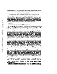
Fig. 7. Fitting a GGX BRDF with SPTDs. The roughness of the BRDF is α = 0.10 and the incident angles are (top) θ o = 0◦ and (bottom) θ o = 75◦ .

5.2

Shading Pipeline

Fitting Procedure. In our rendering examples, we approximate the GGX microfacet BRDF parameterized by an isotropic roughness coefficient α ∈ [0, 1]; this was motivated by the fact that it it is the most widespread BRDF used in the industry [McAuley and Hill 2016]. We adapted the code provided by Heitz et al. [2016] to compute the pivot parameter that produced the best approximation for Equation (14) given a specific input spherical distribution. Since an isotropic GGX material only depends on the elevation angle of the incident direction θo and the roughness parameter α, we only had to fit two parameters for the pivot, namely its elevation angle and its norm. Figure 7 illustrates some fitting results for both a uniform and diffuse input distribution compared to the GGX BRDF as well as the fits from Heitz et al. [2016] using a linearly transformed cosine distribution. Representation and Storage. We precompute our fits inside a 64×64 texture parameterized by roughness α and incident angle θ , fetched with linear interpolation. Our texture stores three coefficients: the pivot elevation angle and its norm, as well as the norm of the fitted GGX BRDF. The size of the texture is 48KB. At runtime, we only need to fetch this texture using the roughness of the material and θo and evaluate the analytic integration of the input distribution D std over the spherical cap д(C ), as given in Equation (15). Choosing the Input Distribution. We experimented with both the uniform and clamped-cosine distributions to fit isotropic GGX materials. We preferred the former over the latter as its tails matched the input BRDFs better, i.e., we use 1 D std = . (16) 4π Note that since the uniform distribution is defined over the entire sphere S 2 , our fits can lead to pivot transformed distributions that leak light under the surface. Fortunately, we can avoid this leaking entirely by restricting the uniform pivot transformed distribution to the hemisphere with an additional spherical cap, as shown in Figure 8. We rewrite Equation (15) into Z Lo = L D (ω) dω, (17) D

A Spherical Cap Preserving Parameterization for Spherical Distributions • 139:7 D

D clipped (hemisphere)

Sphere-light cap

D

D clipped (visibility)

Sphere-light cap

GGX

Uniform SPTD

Fig. 10. Comparison of our technique against ground truth.

Fig. 8. Two-cap integration. Uniform pivot transformed distributions can be analytically integrated over the intersection of two spherical caps. We use this to prevent (top row) light leaking below the hemisphere and (bottom row) specular occlusion with a spherical cap that represents the visibility.

where D = C ∩ H denotes the solid angle formed by the intersection of C and H , the spherical cap oriented towards the normal of the surface and with aperture angle π /2. Thanks to the spherical cap invariance properties of SPTDs, our sphere light integration problem reduces to that of determining the solid angle covered by the intersection of the two caps Z Lo = L D std (ω i ) dω i (18) д(D )

1 =L 4π

Z д(D )

dω i .

(19)

Computing this solid angle can be done analytically using the formula of Oat and Sander [2007], which we provide in Appendix B; Figure 9 shows the result with and without clipping.

5.3

Results

Game Engine Integration. Our technique is easy to integrate into an existing real-time rendering pipeline. Figure 1 shows a scene in which the sphere lights are simulated with our technique in a video-game engine. The scene contains 4 sphere lights and the total rendering time per frame is 16ms at 1920 × 1080 on an NVIDIA GGX

Uniform SPTD without clipping

Uniform SPTD with clipping

Fig. 9. Avoiding light leaking. We prevent light leaking below the hemisphere by clamping the distribution with the spherical cap associated with the upper hemisphere.

Geforce GTX 980 GPU. Note that we also provide animated renderings in our supplemental video that were all rendered in less than 20ms with the same hardware. Performance. We benchmarked our shader by rasterizing a fullscreen quad covering 1920 × 1080 pixels on an NVIDIA Geforce GTX 980 GPU. For a single sphere light source, the shading time is 0.57ms and is independent of the roughness α of the GGX BRDFs we approximate. By adding an additional sphere light, the shading time goes to 1.17ms. This is expected since our algorithm scales linearly with the number of sphere lights. Comparison Against Ground Truths. We provide rendering comparisons against ground-truth results in Figure 1, and Figure 10 (we also provide a more extensive set of comparisons in our supplemental document). We compute the ground truth by importance sampling the GGX microfacet BRDF and we raytrace the sphere lights. At normal incidence, our fits result in materials very similar to the target GGX lobes. At grazing angles however, our fits fail to reproduce the elongated highlights of glossy GGX materials. This error is not due to our fitting method, it is a fundamental limitation of SPTDs: since SPTDs are spherically invariant, we cannot expect them to produce more complex isocontours. This limitation is also clearly visible from the BRDF plots shown in Figure 7. In general, most of the deviations with respect to ground truths will be due to this limitation. Thus, we believe that any future contribution towards extending the behavior of SPTDs to more complex shapes could benefit real-time sphere light shading.

5.4

Specular Occlusion with Bent Cones

In this section, we show how to use SPTDs to incorporate a precomputed representation of visibility within the shading integral known as bent cones [Landis 2002]. General Concept. Whenever distant occlusion is involved in shading, the integrand of the rendering equation writes as a triple product, i.e., Z Lo = fr ⊥ (ω,ω o ) V (ω) L(ω) dω, (20) S2

where V ∈ {0, 1} is the directional visibility at the shading point. Specular occlusion consists in representing the visibility function ACM Transactions on Graphics, Vol. 36, No. 4, Article 139. Publication date: July 2017.

139:8 •

Jonathan Dupuy, Eric Heitz, and Laurent Belcour

sphere light

bent cone

BRDF

(a) Specular occlusion setting

(b) Without spec. occl.

(c) With spec. occl.

(d) Shadow leaking

(e) Light leaking

Fig. 11. Specular occlusion incorporates (c) a rough estimate of visibility for surface shading: (a) the bent cone (drawn in red) modulates the product of the light (drawn in yellow) and the BRDF (drawn in green). Separate integration neglects the correlation between the elements of the shading integral and can lead to (d) shadow leaking or (e) shadow leaking. We show that (c) uniform SPTDs can be used to avoid such artifacts in the case of spherical lights.

by a bent cone, which is a spherical-cap defined by a principal direction (the bent normal) and a spherical area (the ambient occlusion); Figure 11 illustrates the geometry of Equation (23) in the context of specular occlusion. Note that the bent cone representation for visibility was first introduced for interactive rendering [Iwasaki et al. 2012; Klehm et al. 2011; Wang et al. 2009], and is experiencing a renewed interest—under the name of specular occlusion—in the video game industry for shiny surface shading [El Garawany 2016; Jiménez 2016]. Existing Approach with Separability Assumptions. Since the tripleproduct integral of Equation (23) cannot be solved analytically, previous methods approximate this integral by simpler product integrals, for instance: ! ! Z Z 1 V (ω) fr ⊥ (ω,ω o ) dω × L(ω) fr ⊥ (ω,ω o ) dω Lo ≈ f¯ S 2 S2 =

Vf × Lf , f¯

(21)

where f¯ =

Z S2

fr ⊥ (ω,ω o ) dω.

(22)

Intuitively, Vf /f¯ yields the percentage of the BRDF that is not shadowed by occluders, where Vf is usually computed with the intersection of two spherical caps by approximating the BRDF with a spherical cap. The other term L f is the integral of the BRDF over the unoccluded lighting. For instance, in the case of environmental lighting, L f is usually evaluated with a texture fetch in a prefiltered environment map [El Garawany 2016; Jiménez 2016]. In this work, we set L f to the sphere-light shading integral that we computed in the previous section using Equation (15). Limitations of the Separability Assumptions. In the approximate formulation of Equation (21), both the correlations between the BRDF and the visibility and between the BRDF and the lighting are accounted for. However, the correlation between the visibility and the lighting is neglected, which can result in shadow leaking artifacts; Figure 11 (d) illustrates shows an example of shadow leaking artifact. Note that, alternatively to Equation (21), the triple product ACM Transactions on Graphics, Vol. 36, No. 4, Article 139. Publication date: July 2017.

integral of Equation (23) can also be separated into the integral of the product of light and visibility and the integral of the product of light and the BRDF. However, this separation neglects the correlation of the light and the BRDF, which can result in light leaking; Figure 11 (e) shows an example of light leaking artifact. Using SPTDs, we show that we can account for the triple product correlations in the case of spherical lights. Triple-Product Integration with SPTDs. Since a bent cone defines a spherical cap, we can improve the computations of specular occlusion in the case of sphere lighting with uniform SPTDs. Indeed, by approximating the projected BRDF term fr ⊥ with a uniform SPTD in Equation (23) and exploiting the spherical-cap invariance of SPTDs we obtain: Z Lo ≈ D(ω) V (ω) L(ω) dω 2 ZS = D(ω) dω D Z 1 = dω i , (23) 4π д(D ) where D is the intersection of the spherical cap associated with the visibility and the spherical cap associated with the sphere light. This integral has the same form as hemispherical clipping we described in Equation (19). Thus, we can reuse the double-cap integral of Oat and Sander [2007] to compute it; the bottom row of Figure 8 illustrates our approach. Assuming that the bent-cone is the reference representation of visibility, the only approximation introduced by our formulation is the replacement of the BRDF with a uniform SPTD. Hence, we account for the important correlations between the three integrands, thus avoiding light and shadow leaks entirely. Figure 12 shows a few renderings of specular occlusion with varying lighting conditions.

6

SPTDs FOR MONTE CARLO SPHERE LIGHTS

In this section, we show how the spherical cap sampling property of SPTDs can be used to reduce the variance of Monte Carlo renderings.

A Spherical Cap Preserving Parameterization for Spherical Distributions • 139:9 MIS (previous)

Joint MIS (ours)

Fig. 12. Renderings of specular occlusion under a sphere light of varying size.

6.1

Sampling BRDFs

Joint Light Sampling with SPTDs. Figure 13 compares the classic approach for integrating BRDFs over sphere lights against our improved approach made possible thanks to our pivot transformed distributions. The classic approach consists in sampling the BRDF and the light separately and combine them with Multiple Importance Sampling (MIS) [Veach 1998]: the samples are weighted proportionally to the probability density function (PDF) used to generate them. In the case of sphere lights, the best light sampling strategy is to sample a uniform distribution over the spherical cap covered by the light. We propose to improve the light sampling strategy with our pivot approximation of the BRDF. Instead of sampling a uniform distribution over the spherical cap, we sample the pivot transformed distribution over the spherical cap. This produces samples that are distributed closer to the BRDF, which thus results in lower variance. However, these samples are not distributed perfectly according to the BRDF inside the spherical cap since the pivot transformed distribution is just an approximation of the BRDF. This is why we keep the BRDF sampling strategy and combine both with MIS. MIS (previous) BRDF

Light

Joint MIS (ours) BRDF

Pivot-Light

Fig. 14. Variance reduction with joint light sampling. We compare the results obtained with the techniques described in Figure 13 using 32 samples per pixel.

sampling technique is proportional to the inverse of the solid angle of the pivoted spherical cap. If this solid angle is too small, we divide by a value close to 0, which results in numerical instabilities. In our implementation, we detect these configurations by checking if the solid angle of the pivoted spherical cap is smaller than 10−3 and fall back to classic MIS in this case. These configurations are precisely the cases where the result is close to zero (outside the highlights) where variance is low anyway.

6.2

Anisotropic Participating Media

Rendering Equation. Spherical integrals play a fundamental role in the rendering of participating media. Here, we are interested in the local in-scattering equation, which involves a spherical integral of the medium’s phase function fp ≥ 0 against an incident radiance distribution L ≥ 0 Z Lo = L(ω) fp (µ) dω, (24) S2

BRDF

Pivot

Fig. 13. Joint light sampling with SPTDs. (Left) Classic Multiple Importance Sampling combines samples generated with the BRDF and the light separately. (Right) We approximate the BRDF with a pivot transformed distribution and use it to improve the light sampling strategy.

Results. Figure 14 compares results obtained with these strategies. We can see that using the pivot transformed distribution for improving light sampling results in noticeable variance reduction, even though the pivot transformed distribution is just an approximation of the BRDF. Implementation Details. We noticed that in some configurations, our pivot-light sampling is numerically unstable. The PDF of this

where µ = ω o ·ω ∈ [−1, 1] is the elevation of the phase angle, which measures the deviation of the incident ray ω from the direction ω o . In general, this Equation (24) does not have a closed form and is typically integrated with stochastic Monte Carlo. Next, we derive a phase function from a SPTD that can be jointly importance sampled with sphere light sources. The Pivot Phase Function. We derive an anisotropic phase function fp,pivot by transforming a uniform spherical distribution with a pivot point aligned with the direction ω o and with magnitude дp ∈ (−1, 1); its expressions is 2

fp,pivot (µ) =

1 − дp2 1 * + . 4π , 1 + дp2 − 2дp µ -

(25)

The magnitude of the pivot controls the scattering behavior of the phase function, ranging from backscattering through isotropic to forward scattering. ACM Transactions on Graphics, Vol. 36, No. 4, Article 139. Publication date: July 2017.

139:10 •

Jonathan Dupuy, Eric Heitz, and Laurent Belcour

Fitting the Henyey-Greenstein Phase Function. Our pivot phase function has a very similar algebraic expression to that of the Henyey-Greenstein phase function [1941], which is given by 1 − д2 1 , (26) 4π (1 + д2 − 2дµ) 23 where the parameter д ∈ [−1, 1] has the same influence on the scattering behavior as our дp parameter. Since Equation (26) and Equation (25) have very close algebraic expressions, we were able to create very similar renderings by fitting the pivot parameter дp from д with a rational function fp, HG (µ) =

дp = sign(д) Q (|д|),

thanks to the properties of SPTDs. In contrast, with classic phase functions, the phase functions and the lights are sampled separately and combined with MIS. Figure 18 shows that this joint sampling produces lower variance than MIS (more results are available in our supplemental material). MIS (previous) Phase function

Light

Joint MIS (ours) Phase function-Light

(27)

where

0.7489u − 0.6121u 2 . (28) 1 − 0.8409u + 0.0223u 2 Figure 15 shows slices of the phase functions obtained with our fit. Note that the slices do not contain the sin θ Jacobian of the spherical parameterization. Hence, the values at the peaks have much less weight than the side and the angular spread of the distribution is the relevant quantity. Figure 16 shows that our pivot phase functions produce appearances similar to the target Henyey-Greenstein phase functions. Q (u) =

Fig. 17. Joint pivot phase function and light sampling. (Left) Classic Multiple Importance Sampling combines samples generated with the phase function and the light separately. (Right) We use our pivot transformed distribution as a phase function and sample it over the light spherical cap.

MIS (previous)

Joint MIS (ours)

MIS (previous)

Joint MIS (ours)

HG pivot

Fig. 15. Polar plots of the Henyey-Greenstein and pivot phase functions.

д = 0.3

д = 0.7

SPTD

HG

д = −0.5

Fig. 16. Phase function comparison. Our approximation of the HenyeyGreenstein phase function with SPTDs achieves similar appearance.

Joint Phase Function and Light Sampling. Since our pivot phase function matches the behavior of the Henyey-Greenstein phase function, we believe it can serve as a valuable rendering tool, especially given that its importance sampling is more efficient with sphere lights. In Figure 17 we show how we importance sample the phase function over a sphere light. This can be done analytically ACM Transactions on Graphics, Vol. 36, No. 4, Article 139. Publication date: July 2017.

Fig. 18. Joint importance sampling of phase functions and sphere lights. In this figure our pivot phase function matches Henyey-Greenstein with parameter д = 0.9.

7

CONCLUSION AND FUTURE WORK

We introduced Spherical Pivot Transformed Distributions (SPTDs), a new family of spherical distributions with specific analytic properties over spherical caps, such as closed-form expressions, normalization, integration and importance sampling over spherical caps. We applied SPTDs to improve existing sphere-light rendering techniques in both real-time and offline scenarios. We believe that our contributions open up several avenues worth exploring in future work: Coupling with LTSDs. Since our SPTDs produce radially symmetric isocontours, we would like to investigate if it is possible to extend them to support more complex behaviors. We believe combining SPTDs with the linearly transformed spherical distributions (LTSDs) introduced by Heitz et al. [2016] is possible, but finding useful properties that lead to practical rendering techniques remains an open question. Maybe we can find a more general transformation that comprises both SPTDs and LTSDs as special cases.

A Spherical Cap Preserving Parameterization for Spherical Distributions • Other Operators. We do not know whether it is possible to derive other analytic operators that could be useful for rendering applications, such as the inner product or convolution. Parametric Estimation. We would also like to investigate whether it is possible to fit SPTDs to a target distribution by directly extracting a pivot rp instead of using non-linear optimization as we currently do for physically based BRDFs. This was also mentioned in the context of LTSDs, but our problem should be simpler since it has fewer degrees of freedom.

REFERENCES James Arvo. 1995. Applications of Irradiance Tensors to the Simulation of NonLambertian Phenomena. In Proc. ACM SIGGRAPH. 335–342. David Burke, Abhijeet Ghosh, and Wolfgang Heidrich. 2005. Bidirectional Importance Sampling for Direct Illumination. In Rendering Techniques. Eurographics Association, 147–156. Petrik Clarberg, Wojciech Jarosz, Tomas Akenine-Möller, and Henrik Wann Jensen. 2005. Wavelet importance sampling. ACM Transactions on Graphics 24, 3 (jul 2005), 1166–1175. David Cline and Parris Egbert. 2006. Two stage importance sampling for direct lighting. In Rendering techniques. Eurographics Association, 103–113. MichałDrobot. 2014. Physically based area lights. In GPU Pro 5. 67–100. Ramy El Garawany. 2016. Deferred Lighting in Uncharted 4. In SIGGRAPH 2016 Courses: Advances in Real-Time Rendering in Games. Ronald Fisher. 1953. Dispersion on a Sphere. Proceedings of the Royal Society of London A: Mathematical, Physical and Engineering Sciences 217, 1130 (1953), 295–305. DOI:https://doi.org/10.1098/rspa.1953.0064 arXiv:http://rspa.royalsocietypublishing.org/content/217/1130/295.full.pdf Andrew J. Hanson. 2006. Visualizing Quaternions. The Morgan Kaufmann Series in Interactive 3D Technology. Eric Heitz, Jonathan Dupuy, Stephen Hill, and David Neubelt. 2016. Real-time Polygonallight Shading with Linearly Transformed Cosines. ACM Trans. Graph. 35, 4, Article 41 (July 2016), 8 pages. DOI:https://doi.org/10.1145/2897824.2925895 Louis G Henyey and Jesse Leonard Greenstein. 1941. Diffuse radiation in the galaxy. The Astrophysical Journal 93 (1941), 70–83. Udo Hertrich-Jeromin. 2003. Introduction to Möbius differential geometry. Vol. 300. Cambridge University Press. Kei Iwasaki, Wataru Furuya, Yoshinori Dobashi, and Tomoyuki Nishita. 2012. Real-time Rendering of Dynamic Scenes under All-frequency Lighting using Integral Spherical Gaussian. In Computer Graphics Forum, Vol. 31. 727–734. Jorge Jiménez. 2016. Practical Real-Time Strategies for Accurate Indirect Occlusion. In SIGGRAPH 2016 Courses: Physically Based Shading in Theory and Practice. James T. Kajiya. 1986. The rendering equation. In Proc. SIGGRAPH ’86. ACM, 143–150. Brian Karis. 2013. Real Shading in Unreal Engine 4. In SIGGRAPH 2013 Courses: Physically Based Shading in Theory and Practice. Jan Kautz, Peter-Pike Sloan, and John Snyder. 2002. Fast, Arbitrary BRDF Shading for Low-frequency Lighting Using Spherical Harmonics. In Proceedings of the 13th Eurographics Workshop on Rendering (EGRW ’02). Eurographics Association, Aire-laVille, Switzerland, Switzerland, 291–296. Oliver Klehm, Tobias Ritschel, Elmar Eisemann, and Hans-Peter Seidel. 2011. Bent Normals and Cones in Screen-space.. In Vision Modeling Visualization. Eurographics, 177–182. Sebastien Lagarde and Charles De Rousiers. 2014. Moving Frostbite to PBR. In SIGGRAPH 2014 Courses: Physically Based Shading in Theory and Practice. Hayden Landis. 2002. Production-ready global illumination. Siggraph Course 16, 2002 (2002), 11. Pascal Lecocq, Arthur Dufay, Gaël Sourimant, and Jean-Eudes Marvie. 2016. Accurate analytic approximations for real-time specular area lighting. In Proceedings of the 20th ACM SIGGRAPH Symposium on Interactive 3D Graphics and Games. 113–120. Stephen McAuley and Stephen Hill. 2016. Physically Based Shading in Theory and Practice. In ACM SIGGRAPH 2016 Courses (SIGGRAPH ’16). ACM, New York, NY, USA, Article 21. DOI:https://doi.org/10.1145/2897826.2927353 Christopher Oat and Pedro V Sander. 2007. Ambient aperture lighting. In Proc. ACM SIGGRAPH Symposium on Interactive 3D Graphics and Games. 61–64. Pixar. 2016. RenderMan 20 Documentation. https://renderman.pixar.com/resources/ current/RenderMan/rmsPlausibleShading.html#point-and-area-lights. Fabrice Rousselle, Petrik Clarberg, Luc Leblanc, Victor Ostromoukhov, and Pierre Poulin. 2008. Efficient product sampling using hierarchical thresholding. The Visual Computer 24, 7-9 (jun 2008), 465–474. Peter Shirley, Changyaw Wang, and Kurt Zimmerman. 1996. Monte carlo techniques for direct lighting calculations. ACM Transactions on Graphics (Proc. SIGGRAPH) 15, 1 (1996), 1–36.

139:11

John M Snyder. 1996. Area light sources for real-time graphics. Technical Report. Technical report. Andrei Tovchigrechko and Ilya A Vakser. 2001. How common is the funnel-like energy landscape in protein-protein interactions? Protein science 10, 8 (2001), 1572–1583. Eric Veach. 1998. Robust Monte Carlo Methods for Light Transport Simulation. Ph.D. Dissertation. Stanford, CA, USA. Advisor(s) Guibas, Leonidas J. AAI9837162. Jiaping Wang, Peiran Ren, Minmin Gong, John Snyder, and Baining Guo. 2009. AllFrequency Rendering of Dynamic, Spatially-Varying Reflectance. In ACM Transactions on Graphics (Proc. SIGGRAPH), Vol. 28. ACM, 133. JB Wilker. 1993. The quaternion formalism for Möbius groups in four or fewer dimensions. Linear algebra and its applications 190 (1993), 99–136. Kun Xu, Wei-Lun Sun, Zhao Dong, Dan-Yong Zhao, Run-Dong Wu, and Shi-Min Hu. 2013. Anisotropic Spherical Gaussians. ACM Trans. Graph. 32, 6, Article 209 (Nov. 2013), 11 pages. DOI:https://doi.org/10.1145/2508363.2508386 Isaak Moiseevich Yaglom. 2014. Complex Numbers in Geometry. Academic Press.

A

JACOBIAN DERIVATION

Here, we derive the Jacobian of the pivot transformation that we give in Equation (4). This Jacobian measures the rate of change of an infinitesimal solid angle ∂д(ω) on the pivot-tranformed sphere д(S 2 ) with respect to its associated infinitesimal solid angle ∂ω on the original sphere S 2 . Without loss of generality, we assume that the geometry of ∂ω is an infinitesimal disk of radius r 1 ≥ 0. Then, since—as a Möbius transformation—the pivot transformation preserves disks, we know that ∂д(ω) is also a disk. Letting r 2 ≥ 0 denote the radius of ∂д(ω), the Jacobian is then the ratio of the area of these disks ∂д(ω) πr 22 = 2 ∂ω πr 1 ! r2 2 . (29) = r1

д (ω 0 ) ∆д (ω ) д (ω ) rp

ω 0

∆ω ω0

Fig. 19. Geometry for the derivation of the pivot Jacobian.

We can determine the ratio r 2 /r 1 using Figure 19 as follows. According to the intersecting chords’ Theorem, the blue and red triangles are similar, i.e., they are a scaled version of each other. As a result, the ratio between the blue and red edge—which become straight lines when ∆ becomes infinitesimally small—is equal to the ratio of two other similar edges. Thus, letting r 2 = ∆д(ω) and r 1 = ∆ω, we have |д(ω) − rp | r2 = . (30) r1 |ω − rp | Again, from Figure 19, we have |д(ω) − rp | = |д(ω) − ω| − |ω − rp |.

(31)

ACM Transactions on Graphics, Vol. 36, No. 4, Article 139. Publication date: July 2017.

139:12 •

Jonathan Dupuy, Eric Heitz, and Laurent Belcour

The length |д(ω) − ω| can be found from the isosceles triangle formed by the points 0, ω, and д(ω) ω − rp |д(ω) − ω| = 2ω · . (32) |ω − rp | Thus, by injecting Equation (32) into Equation (31) and using straightforward algebra, we find that |д(ω) − rp | =

1 − |rp | 2 , |ω − rp |

(33)

and hence, from Equation (30) 1 − |rp | 2 r2 . = r1 |ω − rp | 2

(34)

Finally, we combine Equation (29) and Equation (34) to obtain Equation (4) 2 ∂д(ω) * 1 − |rp | 2 + . = 2 ∂ω , |ω − rp | -

B

INTERSECTING SPHERICAL CAPS

Exact Formula. The solid angle A ≥ 0 covered by the intersection of two spherical caps C1 and C2 with respective orientations ω 1 ∈ S 2 and ω 2 ∈ S 2 and aperture angles ψ 1 and ψ 2 such that ψ 1 ≤ ψ 2 is [Oat and Sander 2007; Tovchigrechko and Vakser 2001]   2π (1 − cosψ 1 )    A= 0    B  where ψd = cos−1 (ω 1 · ω 2 ) and

if ψ 2 − ψ 1 ≥ ψd if ψ 1 + ψ 2 ≤ ψd otherwise

(35)

B = 2π − 2π cosψ 1 − 2π cosψ 2 ! cosψd − cosψ 1 cosψ 2 − 2 cos sinψ 1 sinψ 2 ! cosψ 1 cosψd − cosψ 2 + 2 cosψ 1 cos−1 sinψ 1 sinψd ! −1 cosψ 2 cosψd − cosψ 1 + 2 cosψ 2 cos . sinψ 2 sinψd −1

(36)

Approximate Formula. In our real-time implementations, we use an approximation of Equation (36) [Oat and Sander 2007] ! ψ 1 + ψ 2 − ψd B ≈ 2π (1 − cosψ 1 )P (37) 2ψ 1 where P (x ) = 3x 2 − 2x 3 . (38)

ACM Transactions on Graphics, Vol. 36, No. 4, Article 139. Publication date: July 2017.