A Spiking Neural Simulator Integrating Event-Driven and ... - IEEE Xplore

This article has been accepted for inclusion in a future issue of this journal. Content is final as presented, with the exception of pagination. IEEE TRANSACTIONS ON NEURAL NETWORKS AND LEARNING SYSTEMS

1

A Spiking Neural Simulator Integrating Event-Driven and Time-Driven Computation Schemes Using Parallel CPU-GPU Co-Processing: A Case Study Francisco Naveros, Niceto R. Luque, Jesús A. Garrido, Richard R. Carrillo, Mancia Anguita, and Eduardo Ros

Abstract— Time-driven simulation methods in traditional CPU architectures perform well and precisely when simulating small-scale spiking neural networks. Nevertheless, they still have drawbacks when simulating large-scale systems. Conversely, event-driven simulation methods in CPUs and time-driven simulation methods in graphic processing units (GPUs) can outperform CPU time-driven methods under certain conditions. With this performance improvement in mind, we have developed an eventand-time-driven spiking neural network simulator suitable for a hybrid CPU–GPU platform. Our neural simulator is able to efficiently simulate bio-inspired spiking neural networks consisting of different neural models, which can be distributed heterogeneously in both small layers and large layers or subsystems. For the sake of efficiency, the low-activity parts of the neural network can be simulated in CPU using event-driven methods while the high-activity subsystems can be simulated in either CPU (a few neurons) or GPU (thousands or millions of neurons) using time-driven methods. In this brief, we have undertaken a comparative study of these different simulation methods. For benchmarking the different simulation methods and platforms, we have used a cerebellar-inspired neural-network model consisting of a very dense granular layer and a Purkinje layer with a smaller number of cells (according to biological ratios). Thus, this cerebellar-like network includes a dense diverging neural layer (increasing the dimensionality of its internal representation and sparse coding) and a converging neural layer (integration) similar to many other biologically inspired and also artificial neural networks. Index Terms— Co-processing CPU–graphic processor units (GPUs), event-driven execution, event-driven neural simulator based on lookup table (EDLUT), real time, simulation, spiking neural network, timedriven execution.

I. I NTRODUCTION One of the main challenges addressed by neuroscientists in the twenty-first century consists of understanding the biological principles of consciousness and mental processes through which we perceive, act, learn, and remember [1]. However, understanding the computing principles involved requires simulations at different levels of detail and at different scales. Within the context of neurorobotics, the possibility of simulating biologically plausible neural networks connected to an active agent, such as a robot [2]–[4] allows us to study behavioral features using body-brain closed-loop experiments. Nevertheless, this imposes strict constraints on computation time Manuscript received November 28, 2013; revised April 9, 2014; accepted July 26, 2014. This work was supported in part by the European Union under Grant REALNET FP7-270434 and in part by the NVIDIA Corporation, Santa Clara, CA, USA. F. Naveros, N. R. Luque, R. R. Carrillo, M. Anguita, and E. Ros are with the University of Granada, Granada 18009, Spain (e-mail: [email protected]; [email protected]; [email protected]; [email protected]; [email protected]). J. A. Garrido is with the Neurophysiology Unit, Department of Brain and Behavioral Sciences, University of Pavia, Pavia 27100, Italy, and also with the Consorzio Interuniversitario per le Scienze Fisiche della Materia, Pavia 27100, Italy (e-mail: [email protected]). Color versions of one or more of the figures in this paper are available online at http://ieeexplore.ieee.org. Digital Object Identifier 10.1109/TNNLS.2014.2345844

(ideally, real-time simulations for perception-action setups with real robots). Studying brain computational principles is the main goal of computational neuroscience, where widely used neural simulators such as GENESIS [5], NEURON [6], Brian [7], and NEST [8] play a fundamental role. These neural simulators usually calculate neuronal dynamics using time-driven simulation methods. These methods divide the total simulation time into small time steps and update each neural-state variable in each time step by means of numerical analysis methods [9]. This iterative updating process represents a heavy computational load, which depends linearly on the number of neurons and neural variables. This computational load may also depend on the number of synapses if we use synapse models with intrinsic dynamics that need to be computed continuously. For synapses where the parameters can be calculated within the event-driven scheme, the computational load would only be slightly affected by the spike propagation and learning rule application processes. Hence, this total computational load makes large-scale neural network simulations in real time almost intractable if directly iterative numerical methods are used. Alternatively, different approaches and techniques have been developed over the last decades: event-driven neural network simulations [10]–[12], neural network simulations in high-performance platforms, such as field programmable gate-array circuits [13], [14], very largescale integration circuits [15], and graphic processor units (GPUs) [16]–[20], and finally, distributed neural network simulations in clusters [21] represent different approaches for large-scale simulation. As a starting point, we chose the open source simulator event-driven neural simulator based on lookup tables (EDLUTs). The very first EDLUT version incorporated only an event-driven simulation scheme into its design [10]. A further step in the technological development of this simulator made it capable of performing hybrid event-and-time-driven simulations [22]. Finally, to take full advantage of new multicore CPU architectures, time-driven methods have been parallelized using OpenMP. This brief describes how EDLUT has been further developed so as to perform event-and-time-driven simulations in a hybrid CPU–GPU platform. This hybrid platform allows computing largescale simulations efficiently on a single computer. While event-driven simulation methods based on lookup tables are always running on CPU, iterative time-driven simulation methods can be run either on CPU (single core and multicore CPU architectures) or GPU, depending on the number of neurons to be computed (a layer of a few neurons can be more efficiently computed on CPU architecture, while GPU architectures are better suited for larger scale neural systems). This brief also presents a comparative study of all these simulation methods operating in our hybrid CPU–GPU simulator for event-andtime-driven simulations.

2162-237X © 2014 IEEE. Personal use is permitted, but republication/redistribution requires IEEE permission. See http://www.ieee.org/publications_standards/publications/rights/index.html for more information.

This article has been accepted for inclusion in a future issue of this journal. Content is final as presented, with the exception of pagination. 2

IEEE TRANSACTIONS ON NEURAL NETWORKS AND LEARNING SYSTEMS

II. S IMULATION M ETHODS IN A H YBRID CPU–GPU A RCHITECTURE According to [23], an event-and-time-driven simulator, such as EDLUT, could be divided into three processing sections: 1) neuronal dynamics (using time-driven and/or event-driven methods); 2) spike propagation; and 3) event queue management. Thus, the computation time can be divided in t_neu_dynamics , t_spike_prop , and t_queue_manag , respectively. In fact, EDLUT uses several techniques to improve the neuronal dynamic computation, thus making this simulator perform better when the neural integration phase 1 prevails over others (2 and 3). Parallelizing time-driven methods in both CPU and GPU would improve the performance of the simulator while maintaining its flexibility and accuracy [19]. This parallelization procedure enables the use of more complex time-driven neuron models and shorter integration time steps, thus obtaining more realistic and accurate results. Furthermore, event-driven methods (based on lookup tables) are best suited for simulating simple neuron models with high levels of performance and precision. Within the field of computational neuroscience, GPUs have also proven useful in speeding up the computation of time-driven simulation methods in some neural networks, thanks to their particular parallel architecture. These GPUs depend on CPU hosts for their operations. When the CPU only initializes the simulation and the GPU computes the whole simulation, some constraints and simplifications have to be considered to parallelize the entire simulation in the GPU properly, as in NeMo [24] and GeNN [24] (i.e., adopting deterministic delay propagation, time-driven simulation, fixedstep integration methods, avoiding event-driven simulation, etc.). Alternatively, when the GPU operates conjointly with the CPU (CPU–GPU platform), such constraints are no longer required since any parallelizable task can be independently performed on GPU, while sequential ones can be performed in CPU as in Brian [7] and our simulator. This means that while EDLUT is running, the GPU updates the neural-state variables in time-driven methods, and the CPU generates, propagates and receives spikes, processes learning rules, and updates the neural-state variables in both time-driven and event-driven methods. To better understand how this hybrid CPU–GPU platform operates, we need to bear in mind GPU pros and cons as well as the implications of establishing a CPU–GPU communication process. The synchronization and communication bridge between the CPU and GPU represent the main bottleneck of this platform. The dialog between these two architectures starts when the CPU commands the GPU to update its time-driven neurons. Before starting to work, the GPU consumes time (this is called synchronization time). Furthermore, there is another overhead time, which occurs when the CPU updates the GPU with the newest variable values obtained (this overhead time is called transfer time). The number of neurons in the GPU must be high enough to compensate both overhead times and then to achieve good speedup rates (compared with a CPU-only processing engine). Therefore, it is clear that when using a hybrid CPU–GPU platform, it becomes crucial to minimize both synchronization and transfer times. The GPU has to implement fixed-step integration methods capable of updating all GPU neurons simultaneously, although the CPU can implement both fixed- and variable-step integration methods. For the comparative study, we have chosen the leaky integrate-and-fire (LIF) neural model because it requires only a few state variables to be implemented. A low number of state variables helps to maintain the synchronization and information transference between CPU and GPU per integration step time to a minimum and also facilitates the model implementation onto lookup tables for event-driven methods.

A. LIF Model The LIF model [26] was implemented using an event-driven method in CPU and a time-driven method in both CPU and GPU. Event-driven methods make use of characterization tables stored in a binary file, which are precalculated in a previous offline stage [10]. They contain the particular lookup tables that characterize the dynamics of each cell and allow updating neural-state variables discontinuously at any simulation time. Time-driven methods make use of a text file containing all the particular parameters, which are required to configure each cell type (i.e., granule cell, Purkinje cell, etc.). The neural state is characterized by the membrane potential (Vm−c ), which is expressed by Cm

d Vm−c = gAMPA (t)(E AMPA − Vm−c ) + gGABA (t) dt × (E GABA − Vm−c ) + G rest (E rest − Vm−c )

(1)

where Cm denotes the membrane capacitance, E AMPA and E GABA represent the reversal potential of each synaptic conductance, and E rest is the resting potential (with G rest as the conductance responsible for the passive decay term toward the resting potential). The conductances gAMPA and gGABA integrate all the contributions received through individual synapses and are defined as decaying exponential functions. The parameters of the neural model and a more detailed description can be found in [26]. As shown in (1), the state of a neuron can be defined using just three state variables. 1) Vm−c represents the membrane potential. When this variable reaches a specific threshold, the neuron generates an output spike. 2) gAMPA and gGABA represent excitatory and inhibitory conductances that modify the membrane potential. These conductances decrease exponentially in each integration step and increase proportionally to the synaptic weight of their connections when an input spike arrives. To solve the LIF neuron model differential equation, a fourth-order Runge–Kutta method was implemented. This differential equation is processed offline in event-driven methods [10] (to build up the neural characterization lookup tables) and online in time-driven methods [22]. In event-driven methods, the size of the lookup table is critical, affecting the accuracy of the simulation. The execution time is also affected because the number of cache failures is higher for large tables, but this impact is small. In time-driven methods, the key factor of the simulation is the integration step size, which drastically affects the accuracy and the execution time. Although in this study we only use this neuron model, our neural simulator also includes other neuron models, such as an LIF neuron model with four synaptic conductance types (available for all the techniques described in this brief), a spike response model (for eventdriven and time-driven in CPU), a Hodgkin–Huxley neuron model (so far only for event-driven in CPU) and so on. B. Implementation As indicated in Section II-A, the neural state of the LIF neuron model can be defined using just three state variables: its membrane potential and its excitatory and inhibitory conductances. In the timedriven scheme, a vector in the CPU or GPU global memory stores the three neural-state variables of each neuron belonging to the same neural model (granule cell, Purkinje cell, etc.). When using CPU methods, these neural-state variables are stored in the CPU global memory. Therefore, with each spike arrival, the CPU updates its corresponding conductance. When using GPU methods,

This article has been accepted for inclusion in a future issue of this journal. Content is final as presented, with the exception of pagination. IEEE TRANSACTIONS ON NEURAL NETWORKS AND LEARNING SYSTEMS

however, these neural-state variables are stored in the GPU global memory and cannot be directly modified by the CPU. In this case, an auxiliary incremental conductance vector with two values per neuron is created in the CPU global memory. The CPU stores the input spike effect for both conductances in this vector (excitatory and inhibitory conductance) at each integration step. When the GPU neurons are updated, the auxiliary vector is transferred from the CPU to the GPU and is added to the conductance values stored in the GPU global memory. Thus, only one single transfer from the CPU to the GPU takes place for each integration step. Moreover, after the GPU neurons are updated, the GPU has to indicate to the CPU which neurons generate an output spike. To do this, a Boolean vector, in which each position represents a neuron, is used. The GPU assigns the value True to the corresponding Boolean vector position when its related neuron has to generate an output spike (its membrane potential reaches a specific threshold) or otherwise assigns the value False. When the neural updating has finished, the Boolean vector is transferred from the GPU to the CPU. Once again, just a single transfer from the GPU to the CPU takes place for each integration step. Finally, the CPU generates the output spikes in the corresponding neurons, inserting them into the event queue [10], [22], which stores all relevant events throughout the simulation process. It is worth mentioning that this CPU–GPU memory management and also the CPU–GPU communication procedure can be used with more complex neuron models (i.e., Izhikevich or Hodgkin–Huxley neuron model). Once the structure of the neural-state variables, their distribution within the memory hierarchies in a hybrid architecture, and the communication protocol between the CPU and GPU have been stated, it is time to define the five steps required to update the neural-state variables of each group of time-driven neurons in GPU. 1) Transferring the auxiliary incremental conductance vector from the CPU to the GPU. 2) Updating the neural-state variables with the new incoming conductance values. This updating is computed according to the neural model associated to each neuron group. If a particular neuron has to generate an output spike, the GPU assigns the value True in its corresponding Boolean vector position or False otherwise. 3) Transferring the Boolean vector from the GPU to the CPU. 4) Resetting the auxiliary incremental conductance vector. 5) Generating the output spikes in the CPU using the Boolean vector (these generated output spikes are stored in the event queue). Nevertheless, using the mapped-memory version (Appendix), the GPU can perform the first and third steps automatically since it is capable of reading and writing CPU memory (the so-called auxiliary incremental conductance vector and Boolean vector). All these processes can be seen in the flow diagram of the new simulator (Fig. 1). The hardware used for running these simulations consists of an ASUS P8Z68-VPRO motherboard, an Intel core i7 2600 K secondgeneration 3.4 GHz CPU (four real cores, eight virtual cores), 32 GB RAM memory DDR3 1333 MHz, and finally, an NVIDIA GTX 470 GPU with 1280 MB RAM memory GDDR5. This GPU model supports mapped memory (Appendix). All the CPU–GPU simulations use this technique. C. Neural Network Topology To measure the performance of the three simulation methods in our hybrid CPU–GPU implementation, we ran different biologically plausible neural network simulations. A neural network representing an

3

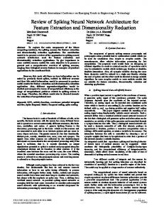
Fig. 1. EDLUT simulator flow diagram. Original flow diagram (white blocks) for event-driven and time-driven methods in CPU and added blocks for the time-driven method in the GPU. These new blocks are executed in the CPU (light-gray blocks) or GPU (dark-gray blocks). The light-gray blocks manage the input information toward the GPU and the output information from it. The dark-gray block updates the neural-state variables in the GPU. An internal spike event [10] generates a spike inside a neuron. A propagate spike event [10] delivers all output spikes after an internal spike event.

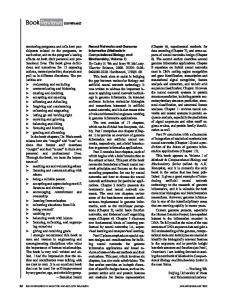
Fig. 2. Neural network representing an abstraction of the granular and Purkinje layers of the cerebellum. The parallel fibers are the axons of the granular cells, which eventually contact different Purkinje cells.

abstraction of the granular and Purkinje layers of the cerebellum [27] was built, as shown in Fig. 2. The cerebellum was structured into microzones [28], each of which included 10 000 neurons distributed in three different layers, as described below. 1) Mossy fiber layer: an input layer consisting of 800 neurons that receive and convey the input network activity to the second layer. This layer is implemented by means of an event-driven method since it is not necessary to update its neural-state variables. 2) Granular layer: consisting of 9120 neurons that mimic cerebellar granule cells. These neurons have four, randomly chosen, input connections from the first layer corresponding to the mossy fiber/granular layer connectivity in biological systems [29], [30]. These input connections have delays of 1 ms. This layer is the most extensive and time-consuming section of the network. We implement this layer using a time-driven method, both in CPU and GPU, and an event-driven method in CPU to compare the performance achieved with each computing scheme. 3) Purkinje cell layer: an output layer consisting of 80 output neurons that mimic cerebellar Purkinje cells. The connections

This article has been accepted for inclusion in a future issue of this journal. Content is final as presented, with the exception of pagination. 4

IEEE TRANSACTIONS ON NEURAL NETWORKS AND LEARNING SYSTEMS

between the granular and Purkinje layers are configured in such a way that each Purkinje neuron has an 80% probability of being contacted by all the granular neurons of its own microzone and a 20% probability of being contacted by all the granular neurons in its two adjacent microzones [31]. These input connections have delays of 3 ms. The number of input synapses (on average) to these neurons is very high (roughly 10 940 synapses per neuron), making an event-driven model somewhat unsuitable for this layer [22]. In addition, the quantity of neurons is not high enough to be run efficiently in a GPU; consequently, in the comparative study in the following sections, this layer is implemented in a CPU using a time-driven method. All the connections are excitatory synapses, there being about 91.2 synapses per neuron in the network on average. This particular network does not use any learning rules, although the simulator can implement different spike-timing-dependent plasticity learning rules. This modular structure, organized in microzones in the cerebellum, can be seen in other areas of the brain (for instance, cortical columns in the cortex [1]). These local neural structures have very intensive local connectivity but sparser connectivity with other microareas (such as neighborhood microzones or cortical columns in the cortex). The input activity supplied to each microzone has been taken from a real simulation of a complete cerebellar model in a manipulation task using six microzones. This activity derives from the sensorimotor (proprioceptor) activity obtained from a three-joint robot arm executing a figure-of-eight-like trajectory in 1 s [4]. The network performance was measured under three different input activity levels which generate 3, 10, and 20 Hz average firing rate over all the neural network activity, respectively, during 10 s simulation time. These three input activity levels were obtained from the original input spike pattern. These new inputs correspond to 3, 6, and 9 executions of the figure-of-eight-like trajectory during 10 s simulation time. For further details, the reader may check and download the EDLUT source code from the project’s official website [32]. The configuration files, neuron models, and input activity files used in this comparative study can be provided upon request. III. R ESULTS This simulator incorporates different simulation techniques, which can work conjointly. As indicated in the previous section, we are simulating a modular three-layer cerebellar spiking neural network where the input mossy fiber layer is always simulated by means of an event-driven method; the granular layer can be simulated by means of an event-driven method in CPU or a time-driven method in both CPU or GPU, and finally, the Purkinje cell layer is always computed using a time-driven method in CPU. The characteristics of each simulation technique at granular layer level are evaluated in two different experiments. 1) Different integration step sizes to be used in time-driven methods and different lookup table sizes to be used in eventdriven methods running in the already established three-layer cerebellar network particularized to a prefixed neural network size. 2) Two fixed integration step sizes and two fixed lookup table sizes to be used in the established three-layer cerebellar network scaled to different neural network sizes. These lookup tables are constructed for the event-driven simulation scheme to obtain an accuracy similar to the time-driven simulation scheme with the two fixed integration steps.

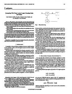
Fig. 3. Ideal speedup rate that could be achieved by the time-driven CPU technique. We show how the speedup rate would behave if the neural dynamics computation time (t_neu_dynamics ) were reduced toward zero and only the spike propagation and queue management had to be processed (t_spike_prop and t_queue_manag ). Simulations run using different integration steps with a neural network consisting of one microzone of 10 000 neurons and 620 000 synapses. Three averaged firing rate neural network activities are used (3, 10, and 20 Hz, respectively).

A. First Experimental Setup We have evaluated the accuracy and performance of the simulation techniques (time-driven methods in CPU and GPU, and event-driven methods in CPU) when adopting these different approaches for the granular layer simulation. The fixed neural network consists of a microzone containing 10 000 neurons and 620 000 synapses. This neural network operates under three defined averaged firing rate neural network activities (3, 10, and 20 Hz). To compare the neural dynamics computation time (t_neu_dynamics ) against the spike propagation and queue management time (t_spike_prop and t_queue_manag ), a profiling of the time-driven CPU technique has been performed. The y-axis of Fig. 3 shows the execution-time ratio between the total simulation time (t_neu_dynamics + t_spike_prop + t_queue_manag ) and the time of the spike propagation and queue management (t_spike_prop + t_queue_manag ). Fig. 3 shows the ideal speedup rate that could be achieved if the neural dynamics computation time (t_neu_dynamics ) were reduced to zero when the time-driven CPU technique is used (see Amdahl’s law [33]). Once the neural dynamics computation time impact has been pondered for the time-driven CPU technique, the aim of this experiment lies in measuring the impact of using different integration steps and lookup table sizes in GPU and CPU, respectively. We use the Van Rossum distance [34] with respect to a 1-µs-integration-step-timedriven simulation to compare the accuracy of the results. We also show the speed-up rate obtained with the time-driven method in GPU and the event-driven method in CPU compared to the stand alone time-driven method in CPU. As shown in Fig. 4(a), while decreasing the integration step size, both time-driven CPU and GPU simulation techniques achieve smaller Van Rossum distances, which means a higher accuracy (the smaller the Van Rossum distance values, the higher accuracy obtained and vice versa). The event-driven CPU simulation technique at the second layer level (granular layer) [Fig. 4(c)], demands an increase of the lookup table size (Table I) from 2.2 to 1750 MB to remain fairly comparable in terms of accuracy with respect to 1 and 0.1 ms time-driven simulations. We should bear in mind that the maximum accuracy that can be reached by the event-driven CPU simulations is limited by the amount of memory available in the CPU for storing lookup tables.

This article has been accepted for inclusion in a future issue of this journal. Content is final as presented, with the exception of pagination. IEEE TRANSACTIONS ON NEURAL NETWORKS AND LEARNING SYSTEMS

5

Fig. 5. Ideal speedup rate that could be achieved in the time-driven CPU technique. We show how the speedup rate would behave if the neural dynamics computation time (t_neu_dynamics ) were reduced toward zero and only the spike propagation and the queue management had to be processed (t_spike_prop and t_queue_manag ). Two fixed integration steps (1 and 0.1 ms) with three averaged firing rate neural network activities (3, 10, and 20 Hz) are used.

B. Second Experimental Setup (Scalability)

Fig. 4. Simulations with different integration step and lookup table sizes (equivalent in accuracy as indicated in Table I) in a neural network consisting of one microzone of 10 000 neurons and 620 000 synapses divided into three layers. The first one is event-driven, the third one is time-driven in CPU, and the second one is computed using the three different simulation techniques: time-driven in CPU (TD CPU); time-driven in GPU (TD GPU); event-driven in CPU (ED CPU); and three averaged firing rate neural network activities (3, 10, and 20 Hz, respectively). (a) Van Rossum distance for both TD CPU and TD GPU with respect to a 1-µs-integration-step-time-driven simulation with tau Van Rossum value = 2 ms [34]. (b) Speedup rate, which is given as TD CPU/TD GPU execution time ratio. (c) Van Rossum distance for ED CPU [for lookup table sizes between 2.2 and 1750 MB (Table I)]. (d) Speedup rate, which is given as TD CPU/ED CPU execution-time ratio.

TABLE I R ELATIONSHIP B ETWEEN THE I NTEGRATION S TEP S IZE OF F IG . 4(a) AND (b) AND THE L OOKUP TABLE S IZE OF F IG . 4(c) AND (d)

We have evaluated how our different simulation techniques evolve in terms of performance when the number of microzones increases. The techniques to be used in the second layer (granular layer) are again time-driven methods in GPU and CPU (adding the possibility of using OpenMP to take full advantage of the multicore architecture that the CPU presents), and event-driven methods in CPU. For that purpose, we have implemented a network with an incremental number of microzones from 1 to 300 microzones (i.e., from 10 000 neurons and 620 000 synapses to 3 million neurons and 274 million synapses). First of all, the time-driven CPU technique demands a profiling (as already made for the first experiment in Fig. 3) to compare and consider the neural dynamics computation time against the spike propagation and queue management computation time. Fig. 5 shows the ideal speedup rate that could be achieved if the neural dynamics computation time were reduced to zero when the time-driven CPU technique is used (see Amdah’s law [33]). As shown in the first four plots of Fig. 6, the shorter the integration step or the larger the neural network in time-driven techniques, the higher the speedup rate of the parallel implementations. This speedup rate reaches a maximum when those tasks to be parallelized in either CPU [Fig. 6(a) and (b)] or GPU [Fig. 6(c) and (d)] are large enough to take full advantage of the hardware. Conversely, event-driven techniques [Fig. 6(e) and (f)] operate quite close to the optimum achievable performance [Fig. 5(a) and (b)]. The inverse relationship between the neural network size and the speedup rate in these figures is caused by the event queue management [10], [22]. IV. D ISCUSSION

Furthermore, a progressive reduction of the integration step size leads the time-driven GPU technique to achieve higher speedup rates [Fig. 4(b)] while maintaining the degree of accuracy that the timedriven CPU technique obtains. The event-driven CPU technique is even able to reach higher speedup rates [Fig. 4(d)] with similar levels of accuracy than the time-driven CPU technique. When comparing both plots [Fig. 4(b) and (d)] with Fig. 3, it is clear that the event-driven technique performs better for the proposed small neural network. The event-driven technique reaches speedup rates quite close to the ideal one, while the GPU parallel hardware (due to the size of this small neural network) is not capable of operating at its maximum performance.

As stated in the abstract, time-driven simulation techniques computed in CPU architectures achieve high performance at high precision when simulating small-scale spiking neural networks. Nevertheless, thanks to brand new features of the current PC architecture, our neural simulator is able to outperform this stand-alone CPU traditional approach using the following. 1) Multicore CPU and GPU parallel architectures for time-driven simulations: the gradual increase of processing units in both architectures motivates the parallelization of processes for highperformance computing. 2) Memory used as a computing resource in event-driven simulations based on lookup tables: the huge amount of available memory in current PCs (up to 32 GB on our hardware) makes this approach a powerful tool when simulating spiking neural networks [10] using event-driven schemes.

This article has been accepted for inclusion in a future issue of this journal. Content is final as presented, with the exception of pagination. 6

IEEE TRANSACTIONS ON NEURAL NETWORKS AND LEARNING SYSTEMS

Regarding the simulation accuracy, time-driven methods, as are well known, only require the decrease of the integration step size to improve accuracy. Under these circumstances, when a high accuracy is demanded, the GPU simulation techniques reach their maximum performance compared with stand-alone CPU simulation techniques. On the other hand, event-driven methods based on lookup tables have to increase the size of their tables to achieve similar accuracy levels to time-driven methods (with shorter integration time steps). The final size of the lookup table depends on the number of neural-state variables needed to define the neural model behavior and the required accuracy. Hence, event-driven methods perform optimally for simple neural models such as the one used in our simulations (LIF) with a medium level of accuracy. On the other hand, time-driven methods, especially when they run in GPU, are better suited for more complex neuron models. With regard to the performance when scaling up the neural network, we have run simulations from thousands of neurons and several hundreds of thousands of synapses to millions of neurons and several hundreds of millions of synapses under different conditions (integration step sizes, lookup table sizes, and averaged firing rate activities). This allows the evaluation of the scalability of our different simulation techniques and the performance of the different processing platforms.

Fig. 6. Speedup rates achieved by three different techniques with respect to the TD CPU (time-driven in CPU) technique: 1) TD CPU OpenMP (timedriven in an eight-multicore CPU) (a) and (b), 2) TD GPU (time-driven in GPU) (c) and (d), 3) ED CPU (event-driven in CPU) (e) and (f). Two fixed integration steps (1 and 0.1 ms) and two lookup tables (2.2 and 1750 MB) to achieve similar levels of accuracy with three averaged firing rate neural network activities (3, 10, and 20 Hz) are used.

The description of how these different simulation methods (eventdriven and time-driven) and simulation platforms (multicore CPU and GPU) are made naturally compatible constitutes the main contribution of this brief (Fig. 1). This hybrid simulator allows us to compute nonhomogeneous simulations in the part of the neural network, which is computed using event-driven techniques (usually neural network layers with either low or sparse activity, independent of their size) while other parts of this neural network (the ones with higher activity or more complex neural models) can adopt time-driven simulation techniques (in CPU for small layers and using GPU for large layers). This means that the best simulation technique can be selected, considering the most suitable part of the neural system, aimed to obtain the best possible performance. Furthermore, the implementation of all these simulation techniques on the same platform allows us to characterize the performance evolution with each approach when different test-bed neural network sizes are simulated. For the evaluation study, we have used a cerebellarlike spiking neural network as a basis [27], which is a good example, as are many others in the brain, where very large layers (such as the granular layer) with sparse activity are interconnected to other smaller layers (such as the Purkinje layer) with a higher average activity.

1) Time-driven CPU with eight cores and GPU versus time-driven monocore CPU: the larger the neural network or the smaller the averaged firing rate activity or the smaller the integration step are, the higher the speedup rate (from ×2 to ×5 using OpenMP parallelism in CPU and from ×4 to ×27 using GPU). 2) Event-driven CPU versus time-driven CPU: the higher accuracy or the smaller the averaged firing rate activity, the higher the speedup rate. Moreover, the smaller the neural network the easier the event queue management and the higher the speedup rate (from ×2 to ×70) when using the event-driven technique. All this provides a clear picture of the relevance of adopting the right simulation technique and computing resources based on the neural network features. As we have shown, today’s technology offers the possibility of simulating millions of neurons on a conventional PC (tens of thousands of neurons can be computed in real time). This is of crucial importance for embedded systems, in which the simulation needs to interact with a robot (body or sensors/actuators). For instance, using a 1-ms integration step (equivalent to a 2.2 MB lookup table in terms of accuracy when using an event-driven scheme) and a 10 Hz averaged firing rate neural network activity, our traditional time-driven CPU technique can simulate, in real time, a neural network consisting of 10 000 neurons and 620 000 synapses. Our parallelized time-driven OpenMP CPU technique can simulate up to 20 000 neurons and 1.53 million synapses in real time. Finally, our time-driven GPU technique and event-driven CPU technique are able to simulate up to 50 000 neurons and 4.13 million synapses in real time. The numbers of neurons and synapses in these examples are related with the neural structure described in Section II. The performance of the event-driven scheme does not depend directly on the size of the network but rather on the number of events to be processed. The maximum neural network size that EDLUT can simulate is constrained by the available RAM memory in the whole system (considering both CPU and GPU RAM memory). Using the cerebellar scheme set out above, we are able to evaluate up to 3 million neurons and 274 million synapses with high average firing rate neural network activity (20 Hz) using 32 GB CPU RAM and 1.28 GB GPU RAM. This simulation on a conventional single computer takes only 987.44 s to compute 10 s of simulation time with our time-driven GPU technique and 1623.96 s with our event-driven

This article has been accepted for inclusion in a future issue of this journal. Content is final as presented, with the exception of pagination. IEEE TRANSACTIONS ON NEURAL NETWORKS AND LEARNING SYSTEMS

7

without mapped memory, especially when the neural network size and/or the integration step size are small. R EFERENCES

Fig. 7. Speedup rate achieved by the mapped memory version of TD GPU compared with the simple version of TD GPU according to the number of neurons. 1 ms (a) and 0.1 ms (b) fixed integration steps are used.

CPU technique. V. C ONCLUSION To develop a powerful simulator capable of dealing with neural networks of very different properties (e.g., neural networks ranging from small to very large, from low and sparse activity to very high activity and able to accommodate from simple to complex neural models), it is mandatory to integrate different simulation techniques (with their own pros and cons) on the same simulator. Throughout this brief, we have described a simulator which integrates different simulation methods (event-driven and time-driven schemes) with different simulation techniques (time-driven methods in CPU and GPU and event-driven methods in CPU) that make use of different processing platforms (single-core and multicore CPU as well as GPU) in the same simulation. We have studied, in detail, the pros and cons of each option. To the best of our knowledge, this is the first simulator that includes all these different simulation alternatives, thus allowing a simulation performance characterization study such as the one presented in this brief. Finally, the next step in our large-scale neural network simulator development will be to implement our simulator EDLUT in CPU/GPU clusters, thus improving the spike propagation and queue management time. At the same time, we intend to work on implementing more complex and realistic neural models (i.e., Izhikevich and Hodgkin–Huxley models), taking advantage of the large computing power of the GPU (these neuron models are defined by more than one differential equation; however, their state variables can still be kept within GPU memory, thus transferring just their conductances from CPU to GPU). A PPENDIX EDLUT has been reprogrammed to make it compatible with Compute Unified Device Architecture for NVIDIA GPUs. The GPU memory should be able to store the neural-state variables of millions or even tens of millions of neurons. The GPU global memory is used to store these variables. To reduce the time-consuming impact of the CPU–GPU communication, our simulation scheme is able to adjust its operation depending on certain GPU features. 1) Legacy GPUs: The CPU writes/reads the GPU global memory. This option is available in all GPU models. 2) Nonlegacy GPUs: Some advanced GPU models incorporate the so-called mapped memory technique. This feature allows the GPU to directly access preallocated sections of CPU memory. The simulator is able to check automatically for the presence of this GPU feature and adopts the best possible option. Fig. 7 shows the differences between the two GPU implementations. The mapped memory version performs faster than the version

[1] E. Kandel, J. Schwartz, and T. Jessell, Principles of Neural Science, 4th ed. Amsterdam, The Netherlands: Elsevier, 2000. [2] R. R. Carrillo, E. Ros, C. Boucheny, and O. J.-M. D. Coenen, “A realtime spiking cerebellum model for learning robot control,” Biosystems, vol. 94, nos. 1–2, pp. 18–27, 2008. [3] N. R. Luque, J. A. Garrido, R. R. Carrillo, O. J. D. Coenen, and E. Ros, “Cerebellar input configuration toward object model abstraction in manipulation tasks,” IEEE Trans. Neural Netw., vol. 22, no. 8, pp. 1321–1328, Aug. 2011. [4] N. R. Luque, J. A. Garrido, R. R. Carrillo, O. J.-M. D. Coenen, and E. Ros, “Cerebellarlike corrective model inference engine for manipulation tasks,” IEEE Trans. Syst., Man, Cybern. B, Cybern., vol. 41, no. 5, pp. 1299–1312, Oct. 2011. [5] J. M. Bower and D. Beeman, The Book of GENESIS: Exploring Realistic Neural Models with the General Neural Simulation System, 2nd ed. Heidelberg, Germany: Springer-Verlag, 1998. [6] M. L. Hines and N. T. Carnevale, “The NEURON simulation environment,” Neural Comput., vol. 9, no. 6, pp. 1179–1209, 1997. [7] D. F. Goodman and R. Brette, “The Brian simulator,” Frontiers Neurosci., vol. 3, no. 2, pp. 192–197, 2009. [8] M.-O. Gewaltig and M. Diesmann, “NEST (neural simulation tool),” Scholarpedia, vol. 2, no. 4, p. 1430, 2007. [9] R. O’Reilly and Y. Munakata, Computational Explorations in Cognitive Neuroscience: Understanding the Mind by Simulating the Brain. Cambridge, MA, USA: MIT Press, 2000. [10] E. Ros, R. Carrillo, E. M. Ortigosa, B. Barbour, and R. Agís, “Eventdriven simulation scheme for spiking neural networks using lookup tables to characterize neuronal dynamics,” Neural Comput., vol. 18, no. 12, pp. 2959–2993, 2006. [11] M. Rudolph-Lilith, M. Dubois, and A. Destexhe, “Analytical integrateand-fire neuron models with conductance-based dynamics and realistic postsynaptic potential time course for event-driven simulation strategies,” Neural Comput., vol. 24, no. 6, pp. 1426–1461, 2012. [12] A. Delorme and S. J. Thorpe, “SpikeNET: An event-driven simulation package for modelling large networks of spiking neurons,” Netw., Comput. Neural Syst., vol. 14, no. 4, pp. 613–627, 2003. [13] E. Ros, E. M. Ortigosa, R. Agís, R. Carrillo, and M. Arnold, “Real-time computing platform for spiking neurons (RT-spike),” IEEE Trans. Neural Netw., vol. 17, no. 4, pp. 1050–1063, Jul. 2006. [14] M. J. Pearson et al., “Implementing spiking neural networks for real-time signal-processing and control applications: A model-validated FPGA approach,” IEEE Trans. Neural Netw., vol. 18, no. 5, pp. 1472–1487, Sep. 2007. [15] H. Chen, S. Saïghi, L. Buhry, and S. Renaud, “Real-time simulation of biologically realistic stochastic neurons in VLSI,” IEEE Trans. Neural Netw., vol. 21, no. 9, pp. 1511–1517, Sep. 2010. [16] A. K. Fidjeland and M. P. Shanahan, “Accelerated simulation of spiking neural networks using GPUs,” in Proc. IJCNN, Barcelona, Spain, Jul. 2010. [17] J. M. Nageswaran, N. Dutt, J. L. Krichmar, A. Nicolau, and A. Veidenbaum, “Efficient simulation of large-scale spiking neural networks using CUDA graphics processors,” in Proc. IJCNN, Atlanta, GA, USA, Jun. 2009. [18] A. Ahmadi and H. Soleimani, “A GPU based simulation of multilayer spiking neural networks,” in Proc. 19th ICEE, Tehran, Iran, May 2011. [19] R. Brette and D. F. Goodman, “Simulating spiking neural networks on GPU,” Network, vol. 23, no. 4, pp. 167–182, 2012. [20] M. Richert, J. M. Nageswaran, N. Dutti, and J. L. Krichmar, “An efficient simulation environment for modeling large-scale cortical processing,” Frontiers Neuroinform., vol. 5, p. 19, Sep. 2011. [21] C. Chen and T. M. Taha, “Spiking neural networks on high performance computer clusters,” Proc. SPIE, Opt. Photon. Inf. Process. V, vol. 8134, p. 813406, Sep. 2011. [22] J. A. Garrido, R. R. Carrillo, N. R. Luque, and E. Ros, “Event and time driven hybrid simulation of spiking neural networks,” Adv. Comput. Intell., vol. 6691, pp. 554–561, Jun. 2011. [23] R. Brette et al., “Simulation of networks of spiking neurons: A review of tools and strategies,” J. Comput. Neurosci., vol. 23, no. 3, pp. 349–398, 2007.

This article has been accepted for inclusion in a future issue of this journal. Content is final as presented, with the exception of pagination. 8

[24] A. K. Fidjeland, E. B. Roesch, M. P. Shanahan, and W. Luk, “NeMo: A platform for neural modelling of spiking neurons using GPUs,” in Proc. 20th IEEE Int. Conf. ASAP, Boston, MA, USA, Jul. 2009. [25] T. Nowotny. GeNN. [Online]. Available: http://sourceforge.net/projects/ genn/, accessed Jun. 2013. [26] W. Gerstner and W. Kistler, Spiking Neuron Models. Cambridge, U.K.: Cambridge Univ. Press, 2002. [27] J. Voogd and M. Glickstein, “The anatomy of the cerebellum,” Trends Neurosci., vol. 21, no. 9, pp. 370–375, 1998. [28] O. Oscarsson, “Spatial distribution of climbing and mossy fibre inputs into the cerebellar cortex,” in Afferent and Intrinsic Organization of Laminated Structures in the Brain. Berlin, Germany: Springer-Verlag, 1976, pp. 34–42. [29] J. Eccles, M. Ito, and J. Szentágothai, The Cerebellum as a Neuronal Machine. Berlin, Germany: Springer-Verlag, 1967.

IEEE TRANSACTIONS ON NEURAL NETWORKS AND LEARNING SYSTEMS

[30] P. Chadderton, T. W. Margrie, and M. Häusser, “Integration of quanta in cerebellar granule cells during sensory processing,” Nature, vol. 428, no. 6985, pp. 856–860, 2004. [31] S. Solinas, T. Nieus, and E. D’Angelo, “A realistic large-scale model of the cerebellum granular layer predicts circuit spatio-temporal filtering properties,” Frontiers Cellular Neurosci., vol. 4, no. 12, May 2010. [32] EDLUT Official Web Site. [Online]. Available: http://edlut.googlecode. com, Jul. 2013. [33] G. M. Amdahl, “Validity of the single processor approach to achieving large scale computing capabilities,” in Proc. AFIPS Conf., 1967. [34] C. Houghton and T. Kreuz, “On the efficient calculation of van Rossum distances,” Netw., Comput. Neural Syst., vol. 23, nos. 1–2, pp. 48–58, 2012.