Medical Image Display & Analysis Group (MIDAG), University of North Carolina at Chapel Hill. ABSTRACT. We present a novel histogram method for statistically ...
IEEE International Symposium on Biomedical Imaging, (ISBI 2006) CD Proceedings: 422-425.
A STATISTICAL APPEARANCE MODEL BASED ON INTENSITY QUANTILE HISTOGRAMS Robert E. Broadhurst, Joshua Stough, Stephen M. Pizer and Edward L. Chaney Medical Image Display & Analysis Group (MIDAG), University of North Carolina at Chapel Hill ABSTRACT We present a novel histogram method for statistically characterizing the appearance of deformable models. In deformable model segmentation, appearance models measure the likelihood of an object given a target image. To determine this likelihood we compute pixel intensity quantile histograms of object-relative image regions from a weighted 3D image volume near the object boundary. We use a Gaussian model to statistically characterize the variation of histograms understood in Euclidean space via the Mallows distance. The probability of gas and bone tissue intensities are separately modeled to leverage a priori information on their expected distributions. The method is illustrated and evaluated in a segmentation study on CT images of the human left kidney. Results show improvement over a profile based appearance model and that the global maximum of the MAP estimate gives clinically acceptable segmentations in almost all of the cases studied. 1. INTRODUCTION The segmentation of 3D deformable objects in medical images is an important and challenging task. Segmentation methods that statistically learn a prior on object shape and a likelihood of an object given an image have several desirable qualities. In this paper, we define an image likelihood measure using quantile histograms of pixel intensities as our basic image measurement and we describe a new method to statistically learn their likelihood. We acquire better generalizability by separately modeling the variation of gas and bone tissue intensities. One category of appearance models is based on the correlation of pixel intensities acquired along profiles normal to the object boundary [1, 2] or from entire object-relative image regions [3]. These methods can be used in conjunction with image filters to summarize information at larger spatial scales and to measure image structures such as texture or gradients [3]. Local methods, however, have difficulty capturing the inter-relations among pixel intensities in a region. Region based methods better capture pixel interrelations by aggregating pixel intensities over global image regions such as object interior or exterior, in one of two ways. In the first, region statistics, such as mean and variance, are either learned during training or functions of them are defined to be minimized [4, 5]. Although the variation of region statistics can be
learned during training, the statistics themselves capture limited information. In the second, each region is represented by a histogram, and a distance to a learned reference histogram is defined [6]. Histograms provide a rich estimate of a region’s intensity distribution but previous work only specifies a reference histogram, and not its expected variation. In this paper, we statistically model histogram variation using a non-parametric histogram representation based on a set of quantiles [7, 8]. This representation allows a distribution to be understood as a point in a Euclidean space via the Mallows distance [9, 10]. Linear operations such as mean and interpolation produce plausible distributions allowing the use of standard statistical tools to model histogram variation. Furthermore, no intensity distribution assumptions are made, making this a flexible tool for many segmentation tasks. Initial image segmentation results using this representation are given in [7]. This paper validates these findings on a large inter-patient kidney data set and describes two enhancements. First, the contribution of each pixel is Gaussian weighted according to its distance to the boundary. This is important due to the often thin layer of fatty tissue surrounding the kidney. Second, the model is modified to take advantage of a priori information regarding the expected probability of gas and bone tissue intensities. Inside the kidney we use the probability learned during training. Outside the kidney, we artificially increase the variance of their expected probability for better generalizability. Our appearance model uses two object regions, inside and outside the kidney. We simplify the probability of the image given the model to be the product of independent, model-relative, image region probabilities. In section 2 we introduce our quantile methodology and construct a statistically learned histogram likelihood. In section 3 we summarize our framework, give segmentation results, and explore ideal results of our appearance model. 2. STATISTICAL MODELING OF HISTOGRAMS We fully train a non-parametric, histogram based appearance model. To do this, we represent intensity distributions as points in Euclidean space in such a way that linear operations such as interpolation and mean produce natural distributions. Principal component analysis (PCA) is then used to compute a histogram’s likelihood. In section 2.1 we construct our histogram representation
Mean & 1st mode
0 CT Value
50
−100
50
−100
50
CT Value
CT Value
50
0 CT Value
0
−100
0 CT Value
50
50
CT Value
−100
Frequency
Frequency
Interior Exterior
Mean & 2nd mode
Frequency
Training Data
0
−100
0
−100
Quantile
Quantile
Quantile
Fig. 1. Histograms and statistics from interior and exterior kidney regions in 39 CT images without gas and bone intensities.
and describe its properties. In section 2.2 we define the likelihood of a histogram and the resulting appearance model. 2.1. Quantile histograms as points in Euclidean space A histogram representation can be understood as a Euclidean vector by considering the similarity measure defined between two histograms that corresponds to Euclidean distance. We use the Mallows distance [9], which was shown by Levina to be equivalent to the Earth Mover’s distance [10]. The Mallows distance can be thought of as measuring the work required to change one distribution into another, by moving probability mass. The position, as well as frequency, of probability mass is therefore taken into account yielding two major benefits. First, over-binning a histogram, or even using its empirical distribution, has no additional consequences other than measuring any noise present in the distribution estimate. Second, this distance measure to some extent mimics human understanding [10]. The Mallows distance between continuous one-dimensional distributions q and r, with cumulative distribution functions Q and R, respectively, is defined as �Z
1 −1
|Q
Mp (q, r) =
(t) − R
−1
p
�1/p
(t)| dt
.
0
For discrete one-dimensional distributions, consider two distributions x and y represented by n quantiles, each storing the average of 1/n of the distribution. Considering these values in sorted order, x and y can be represented as vectors x = (x1 , . . . , xn ) and y = (y1 , . . . , yn ) with x1 ≤ . . . ≤ xn and y1 ≤ . . . ≤ yn . The Mallows distance between x and y is then defined as the (scaled) Lp vector norm between x and y n
Mp (x, y) =
1X kxi − yi kp n i=1
!1/p .
Therefore, histograms are understood as points in an ndimensional Euclidean space in which distance corresponds to the M2 metric. Furthermore, location and scale changes to any histogram are linear. Several families of common continuous distributions are parameterized by location and scale parameters, including the Gaussian, uniform, and exponential distributions. Thus, histograms of each of these families of distributions exist in a two-dimensional subspace linear in their parameters. The Euclidean average of a set of histograms, or the linear interpolation of two histograms, from one of these families of distributions results in a histogram contained within the family. For example, the M2 distance between Gaussian distributions N (µ1 , σ12 ) and N (µ2 , σ22 ) is p (µ1 − µ2 )2 + (σ1 − σ2 )2 . Therefore, linear statistics efficiently capture variation similar to location and scale change in any set of histograms. A weakness, however, for histograms composed of a mixture of multiple underlying distributions, is that changing the mixture amount is a nonlinear operation. 2.2. Histogram likelihood and the final appearance model Our appearance model defines two model-relative image regions, the object interior and exterior. The contribution of each voxel is Gaussian weighted by its distance to the surface. This allows narrow regions to be defined that have larger capture ranges and smoother objective functions during segmentation than equivalent non-weighted regions. In each region, gas and bone intensities are separated using a threshold. The Mallows distance is sensitive to the variation in these intensities due to their extreme values compared to fat and tissue intensities. Figure 1 shows the remaining intensity distributions for a set of kidneys. For each region, we estimate a histogram’s likelihood by constructing a multi-variate Gaussian model. Using PCA, we compute a low dimensional subspace, typically of dimension two or three out of 200. We then measure the expected dis-
0.95 0.9 Training (95.4%) Obj. Function Max (93.7%) Seg. w/ Gas−Bone (91.1%) Seg. wo/ Gas−Bone (90.2%) Profiles (88.3) Landmark Init. (89.0%)
0.85 0.8 0.75
0
5
10
15
20
25
30
35
40
Cases Sorted by Volume Overlap
Ave. Surface Distance (mm)
Volume Overlap (Int/Ave)
1
6 Landmark Init. (2.20) Profiles (2.22) Seg. wo/ Gas−Bone (1.96) Seg. w/ Gas−Bone (1.78) Obj. Function Max (1.27) Training (0.95)
5 4 3 2 1 0
0
5
10
15
20
25
30
35
40
Cases Sorted by Average Surface Distance
Fig. 2. Kidney segmentation results on 39 cases. The legends give each method’s average performance.
tance to this subspace by summing the remaining eigenvalues since during segmentation we expect image regions not typical of the training regions. We also build univariate Gaussian models for the probability of gas and bone tissue intensities. We compute the log probability of each, which is proportional to a sum of Mahalanobis terms. For the histogram Gaussian models, the Mahalanobis distance corresponds to the M2 metric modified to account for the variability in the training data. Figure 1 shows ±1.0 standard deviation along the first two principal directions of variation of each region, which capture 94.8% and 97.4% of the variation, respectively. Training histograms are formed by taking our shape model fit to a manually delineated binary image and computing each voxel’s weight in each region. To define a more accurate optimum for segmentation, voxels are not included where the shape model disagrees with the binary image. However, the expected variation of the actual training segmentations has not been modeled and this can result in segmentations biased towards either the object interior or exterior. Therefore, we normalize each covariance estimate so that the average Mahalanobis distance of the training histograms is its expected value, which is equal to the dimension of the Gaussian model. 3. RESULTS In this section we give segmentation results on the human left kidney. Our data set consists of 39 CT images at an in-plane resolution of 512 × 512 with voxel dimensions of 0.98mm × 0.98mm and an inter-slice distance between 3mm and 5mm. In section 3.1 we discuss our shape model and segmentation framework. In section 3.2 we present segmentation results. 3.1. The segmentation framework We use an m-rep model to describe the shape of the kidney [11]. The object representation is a sheet of medial atoms, where each atom consists of a hub and two equal-length spokes. The representation implies a boundary that passes orthogonally through the spoke ends. Medial atoms are sampled in
a discrete grid and properties, such as spoke length and orientation, are interpolated between grid vertices. The model defines a coordinate system which dictates surface normals and a correspondence between deformations of the same mrep model and the 3D volume in the object boundary region. We perform semi-automatic segmentation by starting with a mean model initialized in a target image using a similarity transform computed from six landmarks. Segmentation proceeds by a conjugate gradient optimization of the posterior of the geometric parameters given the image data. 3.2. Segmentation results We are concerned with the quality of the image likelihood optimum defined by our appearance model and its usability in semi-automatic segmentation. We segment each image using a leave-one-out strategy, 200 quantiles per region, a scale factor of 100 on the variance of the outside gas and bone tissue intensities, and two (three) principle directions for the inside (outside) histograms. Voxel weights are determined using a Gaussian with a standard deviation of 3mm. We compare our segmentations to manual segmentations and those of a profile based method described in [2]. The results are put into context by showing our shape model’s ability to represent the manual segmentations during training. Figure 2 shows that our appearance model without gas and bone information improves upon the initialization and outperforms the profile based method. Including gas and bone information improves results and leads to segmentations deemed clinically acceptable in about 30 of the 39 cases. The results fail, however, to approach training accuracy. To determine if this was caused by our appearance model defining a poor global maximum, we segmented each image starting at the shape model computed during training. In 35 of the 39 cases this optimization found a larger local maximum of the objective function. Figure 2 graphs the segmentation results with the larger objective function value for each image. Assuming the results are representative of the true maximum of the objective function, they show the high quality segmentations defined by our appearance model. 35 of these
(a) 3 of the 4 cases deemed clinically unacceptable.
(b) 3 of the 35 remaining typical segmentations.
Fig. 3. Segmentation results when examining the approximate maximum of the objective function. Each column is a single patient viewed in an axial and coronal slice. The solid contour is the resulting segmentation and the dotted contour in (a) is the training segmentation. Note the contrast enhanced bowel in the first column and the imaging artifacts in the second column.
6. REFERENCES
segmentations were found to be clinically acceptable. Figure 3 shows three clinically unacceptable and three typical segmentations. The first poor segmentation in figure 3 was due to contrast in the bowel, atypical in our set. The second CT image contains reconstruction artifacts.
[1] T F Cootes et al., “Active shape models - their training and application,” Computer Vision and Image Understanding, vol. 61, no. 1, pp. 38–59, 1995.
4. CONCLUSIONS AND FUTURE DIRECTIONS
[2] J Stough et al., “Clustering on image boundary regions for deformable model segmentation,” in ISBI, 2004.
In this paper, we defined a novel appearance model for deformable object segmentation that statistically trains a nonparametric histogram estimate. The proposed model outperforms a profile based appearance model on a given kidney segmentation task. Even more promising are the segmentation results given by the approximate maximum of the objective function defined by our appearance model. 35 out of 39 of these segmentations are clinically acceptable, with two of the failures caused by imaging artifacts. Thus, the appearance model is able to describe the expected image region intensity distributions and their variation. Our next step is to examine additional multi-scale and non-deterministic optimization techniques to more often reach the global maximum of the objective function. We will then validate these findings on a comprehensive intra-patient study of the pelvic region. We also plan on considering several local, model-relative image regions, on modeling intensity distributions as mixtures, and on describing distributions of additional features, such as texture filter responses.
[3] I M Scott et al., “Improving appearance model matching using local image structure,” in IPMI, 2003.
5. ACKNOWLEDGEMENTS
[10] Y Rubner et al., “A metric for distributions with applications to image databases,” in ICCV, 1998.
We thank J. Stephen Marron and Sarang Joshi for discussions on histogram statistics and Gaussian parameter estimation. This work was supported by NIH grant P01 EB02779.
[11] S M Pizer et al., “Deformable m-reps for 3d medical image segmentation,” IJCV, vol. 55, pp. 85–106, 2003.
[4] T Chan and L Vese, “Active contours without edges,” IEEE Trans. Image Processing, vol. 10, no. 2, pp. 266– 277, Feb. 2001. [5] A Tsai et al., “A shape-based approach to the segmentation of medical imagery using level sets,” IEEE Trans. Medical Imaging, vol. 22, pp. 137–154, Feb. 2003. [6] D Freedman et al., “Model-based segmentation of medical imagery by matching distributions,” IEEE Trans. on Medical Imaging, vol. 24, pp. 281–292, Mar. 2005. [7] R E Broadhurst et al., “Histogram statistics of local model-relative image regions,” in DSSCV, 2005. [8] R E Broadhurst, “Statistical estimation of histogram variation for texture classification,” in Texture, 2005. [9] E Levina, Statistical Issues in Texture Analysis, Ph.D. thesis, University of California, Berkeley, 2002.