or non-standard symbols. Others are defined in the text. a h. L. P. PS. 4. 4+ r. R. P. 11. # e. PS. R w radius of earth geopotential latent heat of evaporation of water pressure surface pressure ...... I thank Dr John Green for his .... of some nonlinear baroclinic waves. J. Amos. Sci. 75,. 414-432. Smagorinsky, J. 1960. On the ...
Tellus (1982), 34,211-227
A statistical-dynamical climate model with a simple hydrology cycle By GEOFFREY K. VALLIS, Climate Research Group, Scripps Institution of Oceanography, University of California at San Diego. La Jolla, California 92093, U S A . (Manuscript received June 10; in final form September 16, 1981)
ABSTRACT A zonally-averaged general circulation model is presented, and some experiments with it described. The model is based on the primitive equations of motion, except that the zonally averaged zonal wind is constrained to be in a “spherical geostrophic equilibrium” with the geopotential. The effects of the large-scale eddies on the zonally averaged flow are parameterized using a scheme based on the work of Green (1970):’The solar and infrared radiation schemes allow interaction with the cloud cover predicted via a hydrology cycle. When integrated, the model produces realistic energetics and fields of momentum, temperature and relative humidity. The effects of moisture on the model circulation are examined. Its inclusion intensifies and narrows the upward branch of the Hadley cell, and generally reduces the model ZAPE. The response of the surface temperature to changes in the solar constant is reduced by moisture, especially in low latitudes. Relative humidity is found to have an inverse relationship with surface temperature, if surface albedo is fixed. However, the presence of an ice sheet reduces low level relative humidity. Implications for simple energy-balance models and climate sensitivity are discussed.
1. Introduction Climate modelling is the attempt to understand and simulate the large scale features of the earth-atmosphere system via the construction of mathematical analogs of the real system. General circulation models (GCM’s, see e.g., Somerville et al., 1974) attempt to simulate the atmosphere in as much detail as possible, this limited only by the expense of computer time. Energy balance, or Budyko-Sellers models (BSM’s, after Budyko, 1969 and Sellers, 1969) attempt normally only a prediction of zonally averaged surface temperature. Lying between these in complexity (and perhaps attracting less attention in the literature), are statistical-dynamical models (SDM’s). These are so-called because they attempt to predict from the outset only variables averaged (deliberately rather than of necessity) in space and/or time. It is precisely such fields, rather than their detailed space and time variations, that are of interest in many problems in climatology (e.g., the causes of ice ages, the infiuence of CO,, etc.,. ;;or such problems SDM’s provide, therefore, a more elegant Tellus 34 (1982), 3
approach than GCM’s: aside from their greater economy, they greatly simplify analysis of results and isolation of important mechanisms. We should not, however, view S D M s as rivals to GCM’s, since the latter are in principle more powerful and have more general applicability, but as a complementary tool in climate studies. In this paper a zonally averaged statisticaldynamical model is described and various experiments are performed with it. Zonally averaged SDM’s have previously been constructed by Williams and Davies (1969, Sela and Wiin-Nielsen (1971), Kurihara (1970), Wiin-Nielsen and Fuenzalida (1975), Egger (1975), Saltzman and Vernekar (1971), Ohring and Adler (1978) and Taylor (1980). Zonally symmetric studies have been performed by Hunt (1973, Schneider (1977), Held and Hou (1980) and others. For comprehensive reviews, see Schneider and Dickinson (1974) and Saltzman (1978). Two major problems arise in construction of SDMs. The first is to account for the effects of zonal asymmetries on the mean flow, which appear in the form of Reynolds stresses. Various para-
OO40-2826/82/0302 11-17$02.50/0
0 1982 Munksgaard, Copenhagen
212
0. K. VALLIS
meterizations have been proposed by, amongst An overbar with no subscript will denote a zonal others, Williams and Davies (1965), Saltzman and average. The addition of a subscript implies an Vernekar (1968), Green (1970) and Stone (1972). average over that variable also. The second problem is to parameterize diabatic It is observed and found in primitive equation effects. Although perhaps more progress has been numerical models (e.g., Taylor, 1980) that the made in this area, principally through the demands zonally averaged zonal wind is close to geostrophic of general circulation modelers, problems still equilibrium. This information may be used to remain-largely in the areas of cloud prediction simplify the primitive equation, and eliminate and their radiative interactions, and the for- gravity waves, without seriously impairing the mulation of boundary layer effects. The model usefulness of the resulting set for zonally averaged presented in this paper differs from all previous studies. Thus instead of the full meridional momenmodels in the attempted resolution of these prob- tum equation (namely in log-pressure co-ordinates lems: the eddy fluxes of heat and momentum are av av av u2 ah parameterized using a scheme based on the - + 6- + W- + fti + -tan # + at ay aq a quasi-conservation of potential vorticity and potential temperature by large-scale eddies, and the = eddy correlation terms) diabatic heating makes explicit use of the model predicted hydrology cycle. Also, the set of we use: equations forming the dynamical framework has u2 ah not previously been used in a climate model of this jii + -tan # + - = 0 (1) sort. a aY Section 2 is a description of the basic dynamical This is the only approximation to the primitive set framework of the model. Section 3 discusses the to be made. In particular the Coriolis parameter is physical parameterizations. Sections 4 and 5 are allowed its full latitudinal variation in all terms, the descriptions of some numerical experiments per- static stability is allowed to vary and the metric formed with the model. Section 6 summarizes term ti2 tan #/a is retained. For the purposes of and concludes. numerical integration, the following variables are defined: rn = ( u + Ra cos #)a cos #
2. Model dynamical framework The following list is of only frequently occurring or non-standard symbols. Others are defined in the text. radius of earth geopotential latent heat of evaporation of water pressure surface pressure PS 4 water vapour mixing ratio 4+ saturated value of 4 r relative humidity R ideal gas constant a
h L P
v = up cos #lp, w = w p cos #Ips (rn is the total angular velocity of a parcel of air).
The dynamical set is completed by writing the u-momentum, thermodynamic, continuity and hydrostatic equations (see also Harwood and Pyle, 1975):
am
a
at
ay
-
a .
p l p , cos # -+ - (vm)+ - ( W 4 all
P 11
- 1% PIP,
# e R
latitude potential temperature surface air density earth's rotation rate
w
dqldt
PS
(3) Tellus 34 (1982), 3
213
A STATISTICAL-DYNAMICAL CLIMATE MODEL
av a w -+ - = O
ar
--Re(;) ah
(4)
atl --L
dimensional forms of (2) and (3), which with (7), yields a linear equation for the stream function:
T
mm,
=O
0, (1 + 3 sin2 #)/sin2 4
atl
Note that T / e = (p/p,)” = exp (-Kv) where K = R/C,. S is a diabatic source term. The zonallyaveraged quasi-geostrophic set is a much more severe approximation to the primitive equations than the above set: It is linear, since advection by the mean flow of relative vorticity is omitted; the advection o f f (namely F V ) is neglected; and the static stability and Coriolis parameter held constant. Equation sets similar, but not identical, to (1)-(5) have been used by Harwood and Pyle (1975) and Rao (1973) for middle atmosphere studies. However, they neglected the metric term (U2 tan @/a)in (1). White (1978) pointed out this is energetically inconsistent, and a scale analysis also suggests its omission is not always warranted since the necessary criterion is: ti2 tan 8 4fGa. Although only the geostrophic zonal wind is predicted by (1) through (9,it is advected by the non-geostrophic wind. In this respect the equations are similar to semi-geostrophic set of Hoskins (1975). In order to numerically integrate (1) through (5) eqs. (5) and (1) are first combined to yield a modified spherical thermal wind equation
In the limit of very small Rossby number (6) reduces to the standard thermal wind eqhqtion, namely
am aa
-=
au
Equation (4) is used to define a stream function Y such that
and the equations are non-dimensionalized by choosing arbitrary scaling factors for time, t,, and potential temperature 8,. We choose also y , = a. The non-dimensional form of (6) is now used to eliminate time derivatives between the nonTellus 34 (1982), 3
( + (’)(
c;f;)
HIlm
--
+ ly, --
- -‘OS2
’
p s sin #
8
Ham +-+-
cos2#
COSZ#
Hm, cos2#
(S, + QJ)
where
s =PIPs cos #
(:)dia.atlc
=R
alR0,
The subscripts 7 and # denote derivatives with respect to those variables. Given H,S and Q eqs. (2) (3) and (8) are a closed set. Boundary conditions on (8) of zero normal velocity (Y = 0) are used at the surface, taken at a fixed pressure of lo00 mb, and at 240 mb, the latter crudely representing the tropopause, the higher static stability of the stratosphere inhibiting vertical motion. The model may be global or hemispheric according as y is set to zero at the two poles or pole and equator respectively. The model also includes an equation for the water vapour mixing ratio q, namely P a q a a -cos#-+-(~q)+-(wq) P, at aY as
=s,--
aY a
(-
v’q’cos#-
-
3
--
a:
(-
w’q’cos#-
I) (9)
where S , accounts for the presence of sources and sinks due to precipitation and evaporation from the
214
G.
K. VALLIS
surface. Surface temperature T, is computed via a prognostic equation of the form aT, c,-=-
at
( F , + F~ + FA
Approx. Preswro (mbl level 240 7
5
390
where F,, FL and FR are the net upward fluxes of sensible and latent heat and radiation at the surface, and C, is a heat capacity.
K
i-"Y+
2.1. Numerical integration
J-2
For the integrations to be described the model equations (i.e., (2), (3), (8), (9) and (10)) were finite differenced with a 5 O horizontal grid spacing and 3 vertical levels-the grid is illustrated in Fig. 1, and a hemispheric model used. Time integration is achieved by solving (7) at each timestep by relaxation techniques; the values of V and W determined are used in the momentum, tracer and thermodynamic equation to integrate forward one timestep (by leapfrog) and so on. The balance equation must be elliptic at all times if it is to be solved by successive-over-relaxation. This is violated if
m{-m, e, + m, 8,) > o For m > 0, this implies inertial
(1 1)
or dry-convective instability, which should in any case be prevented by physical parameterizations. This will be described in Section 3. Details of the space differencing schemes are given in the Appendix.
3.1. Large scale horizontal fluxes of heat and
momentum These fluxes manifest themselves mathematically as Reynolds stresses appearing on the right-hand sides of (2) and (3), and are expressed in terms of the mean fields essentially using schemes suggested by Green (1970) and developed further by White (1977). The schemes assume that the eddy flux of a conserved quantity Q may be related to the mean gradient of Q via a tensor array of transfer coefficients K. Thus, regarding potential temperature as a conserved quantity over the timescale of an eddy, we have V I ~= '
ae
ae
- K , - - K,, aY atf
(12)
J
Fig. 1. Grid configuration,indicating locations at which total angular velocity (m)meridional and vertical velocity
(V and W ) stream function ( w ) and potential temperature (8)are held.
where K , and K,, are "transfer coefficients". Applying the transfer theory to quasi-geostrophic potential vorticity, Q, and using the relationship
(13) where B* is a measure of static stability of the form atl/as and is a function of tf only, leads to the following l a ( P U T cos2 0)) ___-
a cos2 0)
3. Physical parameterizations
-
K-2 I JL2
a#
+---
fo
ae a.Y,
B'
ay aq
a
-fo- as (PKvy)
An equation almost identical, but in height co-ordinates, was derived by White (1977) (his eq. (42)). In applying (12) and (14), two problems arise. First our knowledge of the form (and magnitude) of the transfer coefficients (the K's) is scanty. Second, when (14) is integrated over latitude the eddy momentum flux given by the right-hand side will not necessarily vanish for arbitrary K's. One possible solution to both problems is to utilize this integral constraint to yield information regarding the vertical variation of the K's. If eq. (14) is integrated over the model depth and K,, assumed negligible at the upper and lower boundaries, then Tellus 34 (1982), 3
A STATISTICALDYNAMICAL CLIMATE MODEL
a -p (24’ a cos2 4 a#
1 --
tr’ cos2 #)
where
Y=
S K,pdv
We assume the horizontal variation of the K, is separable from the vertical, and the horizontal derivatives of the momentum and potential temperature vary little with height. The constant y is then evaluated at each timestep using the integral constraint of
The vertical variation of the momentum flux is specified to resemble the observed variation-an increasing function of height. Although specification is somewhat unsatisfactory from a theoretical point of view, the observed vertical structure is almost invariant with respect to season. If the horizontal KP, is set proportional to the vertically averaged horizontal temperature gradient,
where K O = 4.8104 m2 s-’ K-I, the maximum value of K{y is then typically 3 x lo6 m2 s-’, in accord with the theoretical estimates of Green (1970) based on the idealized energetics of largescale flows. The horizontal heat flux parameterization is simplified by omitting the smaller term K,, &/aq and choosing the heat flux to decrease with height. The water vapor flux is treated in precisely the same fashion. (This is somewhat ad hoc, and cannot be completely justified on theoretical grounds, since the mixing ratio of a parcel of air is not well conserved on the timescale of an eddy. Its justification will therefore be a posteriori.) Sela and Wiin-Nielsen (197 1) previously used a similar scheme to the one described above, although Tellus 34 (1982), 3
215
without apparently enforcing the integral constraint of (16). In consequence they were forced to subtract a constant value from their zonal wind fields to compensate for the non-conservation of angular momentum by the parameterization scheme. White and Green (1982) discuss this in more detail. Because our knowledge of cyclone-scale eddies in the atmosphere is incomplete, no parameterization theory can expect to be ideal. Simmons and Hoskins (1978) have discussed the inadequacies of linear theory, and Held (1978) in a two-level model found behavior difficult to account for by current parameterization theories. Thus any results which rely on the accuracy of the parameterized eddy fluxes under different conditions would have to be doubted, although I believe the failings of current schemes do not necessarily preclude the usefulness of statisticaldynamical models.
3.2. Vertical heat fluxes Vertical heat fluxes occur in baroclinic eddies and small scale convective processes. The effect of the former is parameterized by setting vertical heat flux equal to horizontal eddy heat flux, multiplied by the isentropic slope. Although linear stability theory suggests that the most unstable trajectory is nearer to half the isentropic slope, non-linear numerical integrations (Simmons and Hoskins, 1978) and observation (Oerlemans, 1980) suggest a larger value for the trajectory is appropriate over the full life cycle of baroclinic eddies. Convective heat fluxes occur in the model whenever the static stability falls below a critical value, and are proportional to the deviation from that value. Thus
where ( W a q ) , is a critical value, discussed in Section 3.8. K, is given the value (in height coordinates) of 75 m2 s-l, implying a timescale of -3 days for disturbances half the depth of the troposphere. These schemes are sufficient to prevent the occurrence of hyperbolic regions in (7) via convective instability. The explicit prevention of inertial instability was found unnecessary.
216
G. I (T, (aT/aq)Sq)than when T, < (T, - (aT/aq)Sq).(See for instance, Gadd and Keers, 1970.) Thus it is incorrect to write, for the zonally averaged flux
since F, > 0, even when T, = T, - (aT/aq)dq.This is roughly accounted for by using for the zonally averaged flux
where A is tuned to give the correct globally averaged value for the sensible heat flux. With K , = 3 cm/s, a value for A of 20 W m-z is found. If F, < 0, K H is reduced by a factor of five. Clearly, the addition of A is equivalent to choosing a different value for (aT/aq),but in (21)the critical lapse rate is the same function of temperature as is used in ( 1 7 ) and not a tunable parameter. Evaporation is parameterized along similar lines, except there is no “critical lapse rate” in the constant flux layer and no additional term is found necessary. Thus Tellus 34 (1982), 3
FL
= LP, kL(?, - &)
217 (22)
4, is the saturated mixing ratio at a temperature T, and lo00 mb. 4; is the model predicted value at level 2. K Lis a constant with the value 0.6 cm s-’. 3.6. Condensation In three-dimensional GCM’s a common procedure is to calculate mixing ratio and temperature assuming no condensation. If saturation is exceeded mixing ratio and temperature are simultaneously adjusted to restore some critical value of relative humidity, often simply unity. For a zonally averaged model this recipe is inappropriate since the observed precipitation rate is non-zero at all latitudes, for all seasons, whereas zonally averaged relative humidity has maxima in the tropics and in mid-latitudes and is certainly less than unity everywhere. The fact that the rate of precipitation varies meridionally in the same sense as zonally averaged relative humidity and absolute humidity suggests a condensation criteria of the following form
. 4+
-
P=-(r--r,)
r>r,
P=O
r < r,
r
(23)
where r, and r are constant. Values currently used are 0.56 and 1 day, respectively. Halving or doubling the value of r changed the condensation rate by nowhere more than 10%. Raising or lowering the value of r, raised or lowered values of atmosphere relative humidity more or less uniformly without changing the meridional or vertical distribution. This consequently lowers or raises evaporation and hence precipitation, but the distribution of relative humidity and precipitation are relatively insensitive to the numerical values of these parameters. It is clearly not possible to explicitly simulate the distribution of latent heat occurring in cumulus and cumulo-nimbus, but their effects on the large-scale flow are certainly not negligible. Thus whenever condensation occurs in a column in which convection is occurring (i.e., there are non-zero eddy convective heat fluxes as described in Section 3.2), the latent heat of condensation is distributed in the vertical such that the heating rate (deg/day) at all levels is equal. This is roughly as observed by Yanai et al. (1973).
218
G. K. VALLIS
1.0 1
0.8
i
1
W 0.6 -
e
4. Some numerical integrations
V
0
s
=)
0.4
-
V
0.2 -
0
adiabatic lapse rate provides a useful contrast with the dry model.
20
40
60
80
100
RELATIVE HUMIDITY (O/o) Fig. 3. Cloud-relative humidity parameterization used at low (L) and mid (M) k v e k High cloud is fixed at a fractional coverage of 0.1.
3.7. Cloud cover In an observational study Smagorinsky (1960) noted a close, linear relationship between fractional cloud cover and relative humidity. Since then various GCM’s have used similar relationships (e.g., the NCAR GCM: Schneider et al., 1978; the BMO GCM: Gadd and Keers, 1970). In this model, a linear relationship between low and middle fractional cloud cover and relative humidity was used (see Fig. 3). High cloud was held fixed at a fractional coverage of 0.1 since there is less basis for a similar relationship for high, cirrus type cloud. These relationships were used to provide a fractional cloud cover for the control experiment (CW).
3.8. The critical lapse rate and the dry model The model described above is fully moist in that it calculates the water vapor mixing ratio, and the condensation and evaporation enter into the thermodynamic equation. The critical lapse rate for this model is set at the local wet adiabatic lapse rate. The model may be made essentially dry by setting the latent heat of condensation to zero. However, in order to avoid gross changes in the vertical temperature structure, and to prevent dry convective instability, the critical lapse rate is set at 6.0 K/km, instead of the dry adiabatic lapse rate (g/C,,).In the moist model it may be more realistic to use a critical lapse rate varying between the wet and dry lapse rates, perhaps as a function of relative humidity. However, the adoption of the wet
This and the next section describe various experiments performed with the model. First we describe integrations performed with the present value of the solar constant for the moist and dry models. Then the solar constant is allowed to change, but surface albedo is kept fixed. Finally we examine the effect of allowing the high latitude surface albedo to change. The solar zenith angle for all experiments is that of the mean annual average, and the model run in all cases until a steady state is reached (requiring about 80 seconds cPutime on a CDC 7600 for 2 years real-time The experiments are summarized in Table 2.
4.1. Integrations for wet (CW) and dry (CD) models The moist model is integrated until a steady state is reached (experiment CW). Using the cloud distribution found in this integration the dry model is integrated (experiment CD). The integration C W is expected to most closely match the present climate of the earth; fields for C D are illustrated only when differing notably from CW. 4.2. Temperature and zonal wind fields The temperature fields are illustrated in Fig. 4. For C W they are certainly realistic-note the flat temperature gradient in low latitudes, maintained primarily by the Hadley circulation, and the slight poleward decrease of the low level lapse rate. The high polar albedo produces a cold surface but the higher temperature of the lower troposphere is paintained by the parameterized influx of heat from lower latitudes. Table 2. List of experiments Name
Description
CW CD CW5 CD5 SAH SAL
Moist control model As for CW but dry As for CW but solar constant reduced by 5% As for CW5 but dry Moist: high polar albedo Moist: low polar albedo Teilus 34 (1982), 3
219
A STATISTICALDYNAMICAL CLIMATE MODEL
=-\
adiabatic lapse rate with falling temperature is acting to produce the opposite effect. The zonal wind for the surface and 5 0 0 mb are illustrated in Fig. 5. The lack of upper level equatorial easterlies is the main deficiency, which may in part be due to the imposition of thermal wind equilibrium; a reversal of the temperature gradient is then needed for easterlies. (Upper level easterlies are found with asymmetric hemispheres in a global version of the model. Schneider (1977) also discusses this.) The surface winds are easterly in low latitudes, westerly in mid-latitudes and with weak polar easterlies. Precisely the same form is found for the dry model, but the larger temperature and thermal wind gradients produce larger transfer coefficients. The momentum transport and hence surface wind are consequently somewhat bigger.
\
0
2 0 4 0 6 0 8 0
4.3. Mean meridional circulation and heat balance The mean meridional circulation is illustrated in Fig. 6, and is dominated by the Hadley and Ferrel cells. The model Ferrel cell owes its existence entirely to the parameterized effects of the eddy heat and momentum fluxes. In the upper two model levels the momentum balance is found to be approximately
LATITUDE Fig. 4 . Model temperature fields for moist and dry models, for surface (S), low (L), mid (M) and high (H) levels. Solid line is for CW, broken line for CD.
The meridional temperature gradient in the dry model is somewhat larger since energy can now only be transported poleward in the form of sensible heat. Notice also the difference in temperature between the ground and lowest atmospheric model level. The radiation surplus at the ground can only be balanced by sensible heat flux in the dry model, whereas about 80% of the deficit is transported by latent heat in the moist model. A polewards decrease in lapse rate is more marked here because in the moist model the increase in wet
l
k
The Hadley cell is directly driven largely by the meridional gradient of diabatic heating, both sensible and latent, and the momentum balance resides between the Coriolis force and the advection of relative momentum. A quasi-geostrophic model, on the other hand, requires internal friction or eddy fluxes of momentum to produce a mean meridional circulation since a (non-zero) steady state can arise only through the balance of the 1
I 0
1
1
2
1
0
1
1
1
4 0 6 0 LATITUDE
1
1
8
I
1
1
0
Fig. 5. Zonal winds at surface and mid level (S and M respectively). Solid line is for CW, broken line for CD.
Tellus 34 (1982), 3
a
fv = - (rncos* 4) a cosz 4 a(
I LATITUDE
Fig. 6 . Stream function for mean rneridional circulation for CW. Units are lolokg s-'.
-I
meridional circulation (Fig. 7). In fact, a slight minimum in the vertically averaged heat balance of CW is apparent-a feature also of some observations. Fig. 8 graphs the average vertical velocities of the moist and dry models. The upward branch of the Hadley cell is narrowed and strengthened by the effects of moisture, although the total width is unaltered.
,---
1.0
>r
0
7 3 0 Y
- 1.0 SOURCE
-
EDDY
1.0 -
-I 8 0
/--\ /
/'
2,
Y
-
-1.0
-
I
\
,.-
'
/
'/
' A \
Fig. 7 . Vertical mean heat balance expressed in degrees/ day, as a function of latitude in CW (moist) and C D (dry). The contributions are defined as:
4.4. Energetics
It was noted above that the meridional temperature gradient of the dry model was slightly larger than in the moist model. The energetics illustrate the same effects more dramatically (Fig. 9). The wet model appears very much less energetic: the ZAPE is smaller, and its generation and conversion to EAPE smaller. The ZAPE is smaller simply because of the smaller temperature gradient (ZAPE is proportional to the square of the zonally averaged temperature variance on an isobaric surface). The generation of ZAPE is proportional to the correlation b e t w m e m p e r a t u r e ( T ) and is an diabatic heating (S)-T*S*-where isobaric average and * a deviation from such an average. In the moist model latent heat is transferred polewards before release, so reducing this correlation. In the dry model some of this transfer is essentially added to the transfer of sensible heat, thus increasing ofZAPE to EAPE (proportional to F*(a/@)vT*).
-
vortex stretching and eddy momentum flux terms in the vorticity equation. The condensation of moisture in the upwards branch of the Hadley cell does produce a more intense meridional gradient of heating in the moist model, the consequence being a stronger contribution to the mean heat balance from the mean
0'3
-0.3 -Oa2
1
\MOIST (CW)
1
Fig. 8. Vertical mean vertical velocities for CW (solid line) and C D (broken line).
Fig. 9. Lorenz energy cycle. Figures for CW are without brackets. Figures for C D are in square brackets. Observed figures (from Oort, 1964) are in curly brackets. Units of energy are lo5 J m-'. Units of transfer are W
m-'. Tellus 34 (1982), 3
22 1
A STATXSTICALDYNAMICAL CLIMATE MODEL
4.5. Moisture fields for CW Water vapor mixing ratio is determined mainly by temperature, and is not a sensitive test of a model's ability to predict moisture field. A more suitable field is relative humidity. This is pictured in Fig. 10, and the corresponding precipitation and evaporation in Fig. 11 and cloud field in Fig. 12. The observed meridional response is reasonably well reproduced. The maximum on the equator and minimum in the subtropics arise from the effects of the mean circulation, and the mid-latitude peak is due to the polewards eddy flux. Fig. 13 illustrates how the mean circulation is dominant in low latitudes in transforming water vapor equatorward RELATIVE HUMIDITY
-'
--1
/
cr
W
>
0.6
L3 3
0
6
0.4
J
a
z
0
F 0.2 V
a
cr
40 60 80 LATITUDE Fig. 12. Computed fractional cloud cover at low and mid levels (L and M), and the total cover (T, which includes the effects of a constant, 0.1, fractional high cloud cover).
20
0
--
I
1
b , 3 1y 9 2 v)
E a Y
IY
' 0 -1
-2
20 40 60 LATITUDE o
10
M
ro
30
M
60
ro
m
90
LATITUDE
Fig. 10. Latitude height distribution of relative humidity. The observed values are from London (1957) for winter. (Other seasons are qualitatively very similar).
I\
2.0 L
)r
\
E
I1..o 5
0.5 -
"\.
PRECIP. \.
sl
0 10
30 50 70 LATITUDE
90
Fig. 11. Precipitation (solid line) and evaporation
(broken line) in CW. Tellus 34 (1982), 3
80
Fig. 13. Computed vertical mean polewards flux of water vapor by eddies (dashed line) and the mean flow
(solid line) Observed values are marked by circles (from Oort and Rasmusson, 1971).
(and up gradient). The vertical structure of the relative humidity field is more difficult to understand, since in the absence of any eddy vertical velocities and parameterized vertical transport of water vapor, the observed mid-tropospheric minimum is obtained. The imposition of a lid at 240 mb enforces maximum vertical velocities in mid-troposphere, and this appears sufficient to produce the relative humidity maximum. Further research is clearly needed to evaluate the effects of the precipitation criteria and the importance of vertical eddy transports. It should also be pointed out that the various observations of upper level relative humidity are probably subject to large error.
222
G. K. VALLIS
The above integrations show that the moist model can reproduce with a fair degree of accuracy the observed zonally averaged atmospheric circulation and that the inclusion of moisture does not qualitatively alter the model circulation. The next section, however, will show that the detailed responses of the two models to a change in solar constant have marked differences.
6
Y
-
b
a
4
2 ' MOIST
5. Changes in forcing
P
5.1. Solar constant
Although changes in the solar constant of several percent may never have occurred, its variation is a useful device in modeling since it is a sure means of producing different climatic regimes in which the relative roles of various physical processes can be assessed, and intercomparison between models facilitated. The next subsections describe the major changes occurring in the moist and dry models when solar constant was reduced by 5%. In general very similar behavior, but of opposite sign where appropriate, was found for a rise in solar constant of the same magnitude. 5.1.1. Temperaturefields. Fig. 14 illustrates the temperature changes caused by a 5 % lowering of the solar constant. Very similar behavior but of opposite sign was found for a rise in solar constant of the same magnitude. In the dry model the temperature changes show a general decrease poleward, due to the fact that the change in magnitude of the insolation also decreases polewards. The ground temperatures have everywhere changed more than atmospheric temperatures. A simple argument explains the cause: Suppose we describe the earth-atmosphere system by two temperatures T, (which might be the 500 mb temperature, say) and Tg, the surface temperature. Assume the atmosphere to be transparent to solar radiation, but opaque to infrared radiation emitted by the surface. Radiative-convective equilibrium demands, for the atmosphere to be in energy-balance 0 = Zg(Tg)- Ia(T,) + f W g 9 T,)
2 0 4 0 6 0 8 0 LATITUDE
OO
(24)
where Z, is the total infrared emission of the atmosphere, Z, = aT:, andf(T,, T,) represents the exchange of sensible and latent heat between atmosphere and ground. From (24)
a
2[ DRY
0
1 20 40 60 80
0
LATITUDE Fig. 14. Temperature changes at surface and low, mid and high levels induced by a 5 % change in solar constant in moist and dry models.
_dT,_ - dZgldTg + (af/aTg), dT,
dl,/dT, - (aflaT,),
If (af/aT,), = -(af/aT,),, which may hold approximately if we are describing the exchange of sensible heat by bulk-aerodynamic type laws, then dT,/dTg is less or greater than unity according as dZ,ldT, is less or greater than dZ,/dT,. Now, dZg/dTg 5.4 W m-* K-' (at 288 K) whereas using Smagorinsky's (1963) parameters, dZ,/dT, typically ranges between 6 and 9 W m-' K-'. Thus dT,/dT, is less than unity. In the presence of water vapor we clearly do not have (af/aT,JTI= (-af/aT& because of the presence of water vapor. The simplest possible way to include moist effects in this framework is through a linear formula of the form
-
Tellus 34 (1982), 3
A STATISTICAL-DYNAMICAL CLIMATE MODEL
where a, b and c are constants. It is now quite possible to have ( a f / a T , ) , > -(af/aTa)T8 since aq,/aT, > aq,/aT, for qs > 4,. Physically, as we reduce the solar constant, and hence temperature, evaporation falls rapidly and surface and atmospheric energy balance is maintained only by an increase in sensible heat transfer, and an increased lapse rate is demanded. Away from the surface the increase in wet adiabatic lapse rate with decreasing temperature is responsible for the changes in vertical temperature structure observed in the wet model. Held (1978) obtained broadly similar results using a two-level three-dimensional primitive equation model, although his “dry” model still contained surface evaporation and so his effects were entirely due to changes in the wet adiabatic lapse rate. That the simple argument above can qualitatively explain the gross features of the variation with latitude of the vertical temperature structure changes certainly points to the fact that vertical subgrid energy fluxes play an important role in determining the surface temperature response. An effective parameterization of the large scale horizontal fluxes is necessary, however, in order to produce the meridional variations of temperature upon which the vertical parameterizations act. The precise interplay between the two parameterizations is currently the object of study. Even in the absence of ice-albedo feedback, which is generally considered to amplify high latitude changes, the low latitude surface response
0
20
40
60
is seen to be reduced by moist effects. Unless such effects can be parameterized within the framework of Budyko-Sellers models their quantitative results should clearly be regarded with caution. 5.1.2. Moisture fields. The relative humidity changes in the moist model are depicted in Fig. 15. A decrease in solar constant is accompanied by an increase in relative humidity (and hence cloudiness, if the two are related). Recent experiments with GCM’s have given generally similar results. Schneider et al. (1979) obtained decreases in relative humidity of approximately 1% per degree Celsius rise in sea surface temperature, although they do not discuss its distribution. Roads (1978a) obtained similar behavior in a more detailed model of the hydrology cycle. Wetherald and Manabe (1980) also found relative humidity decreasing with increasing temperature in the mid- and uppertroposphere, although at low levels especially in high latitudes relative humidity increased with increasing temperature. These investigators explained their results in terms of an increase in the intensity of the hydrology cycle with increasing temperature, so causing an increase in the variance of the deviation of vertical velocity from its zonal mean. Under conditions where cloud cover already exists in regions of descent, this causes more drying in regions of descent than moistening in regions of ascent, and a lower area mean relative humidity. Such a mechanism does not exist in a zonally averaged model, and other processes are responsible. We noted above that a decrease in the solar constant demands a greater lapse rate. Thus if the vertical profile of mixing ratio remains more or less unchanged, atmospheric relative humidity will rise, a notion also consistent with the results of Roads (1978b): Defining scaled evaporation as the ratio of surface saturated mixing ratio (q:) to an atmospheric saturated mixing ratio (4:) then, Roads showed, mean atmospheric relative humidity will generally increase if scaled evaporation increases. Now, if temperature falls then scaled evaporation will increase, since q:/qz is a decreasing function of temperature, and so relative humidity rises. If lapse rate increases, the scaled evaporation and relative humidity further increase.
80
LATITUDE Ffg. 15. Percentage increase in relative humidity due to 5 % fall in solar constant.
Tellus 34 (1982), 3
223
5.2. Changes in high latitude albedo It is the above described process which is dominant in this model in producing the general
224
G. K. VALLIS
decrease in relative humidity with increased temperatures. It is presumably also operative in general circulation models. Wetherald and Manabe (1980) did, however, find that the high latitude low level cloud cover increased with increasing temperature, this in a region where eddy vertical velocity changes were small. This behavior occurred largely over a region where surface albedo decreased rapidly (due to the retreat of the ice line) causing surface temperatures to rise dramatically. To examine the effects of changing surface albedo, two experiments were performed which differed only in surface albedo. Experiment SAH has a high (0.7) albedo polewards of 65O, but the same as that illustrated in Fig. 1 equatorwards. SAL has a low (0.2) albedo polewards of 65O but identical SAH equatorwards. Fig. 16 illustrates the temperature differences between the two integrations, and Fig. 17 the relative humidity differences. The effect of a high
albedo is, as expected, to lower surface temperatures significantly, but the reduction of atmospheric temperatures is moderated by the parameterized influx of heat from lower latitudes. Thus a much stronger low level inversion arises in SAH. Surface evaporation is much smaller because the lapse rate is also smaller; a fall in the low level relative humidity occurs. Mid-level relative humidity shows a small increase. It is interesting to note that just equatorwards of the latitude where albedo has changed surface temperature changes are smaller than the lower troposphere changes because of the lateral transport of heat in the atmosphere, and here low level relative humidity is higher in SAH than SAL, due to the mechanisms explained in Section 5 .
6. Concluding remarks
This paper has described a highly parameterized climate model and some model integrations. 10 As far as possible, the eddy flux boundary layer and diabatic heating parameterizations all derived from physically or dynamically based theories. Y With these schemes, a realistic simulation of the L 5 4 zonally averaged atmosphere was posible with the moist model. However, there are probably two areas in which our ability to parameterize the 0 relevant process is still open to much improvement. 1 1 1 1 1 1 1 1 l (i) The large scale eddy flux parameterizations. It 50 60 70 80 90 would also be useful in this context to understand LATITUDE to what extent present theories are inadequate, Fig. 16. Temperature difference between SAL (low high and to what extent they have predictive ability. latitude albedo) and SAH (high high latitude albedo). The parameterization of eddies in the stratosphere is necessary if the model is to be extended vertically. (ii) Parameterization of cloud fields. The 5 parameterization of precipitation was undeniably empirical, although apparently giving good results. A more dynamically or physically based scheme is needed. Similarly, the relationship of zonally averaged cloud to zonally averaged moisture fields is not entirely clear. For example, most obser-5 1 I vations of the cloud field (e.g., CIAP, 1975) tend to show a maximum in mid-to-high latitudes at a value higher than the equatorial maximum, even 50 60 70 80 90 though the equatorial relative humidity is often LATITUDE Fig. 17. As for Fig. 16, but percentage change in relative higher. This is most likely due to the greater humidity. Positive values mean relative humidity was variance of eddy vertical velocity at the equator (at higher for SAL. least in GCM’s, e.g., Wetherald and Manabe, 1980) A
c
1
Tellus 34 (1982), 3
225
A STATISTICAL-DYNAMICAL CLIMATE MODEL
which will tend to prevent cloud cover from rising much above 50%. This may be very difficult to parameterize in a zonally-averaged model. These inadequacies may preclude the use of SDM’s from yielding quantitative results regarding the climates sensitivity. Yet their simplicity may lead to important insights into mechanisms possibly obscured in more complex models. To this end experiments were performed first to evaluate the influence of latent heat release in the model circulation. The model circulation was not qualitatively altered, although detailed differences did arise. The wet model was less energetic, in response to a reduced meridional temperature gradient, and the upward branch of the Hadley cell was narrowed and strengthened. However, the response of the wet and dry models to a change in solar constant was radically different. The presence of moisture acted to reduce significantly the change in surface temperature (and so alter the lapse rate) at low latitudes, compared with the dry response. This effect is clearly very difficult to model in Budyk-Sellers models, since these implicitly assume a lapse-rate unchanging with time. The effect of surface temperatures responding less than atmospheric temperatures is to produce an inverse relationship between cloud cover, or more strictly relative humidity, and temperature. However, this inverse relationship in high latitudes is modified if surface albedo is allowed to change, for this amplifies surface temperature changes more than atmospheric changes. The effect of increasing high latitude surface albedo, was to decrease the evaporation and relative humidity above the “icesheet”, because the surface temperature change was much larger than the atmosphere’s. This effect may be the cause of the increase in low level high latitude cloud found by Wetherald and Manabe (1980) when solar constant was increased by 6%. If this is so then clouds would feedback positively on any change in solar constant. In low and mid-latitudes any increase in cloud cover following a reduction in solar constant would reduce temperature further. In high latitudes the presence of a high surface albedo means the effect of clouds in the infrared is dominant and the positive feedback effects of an increase in icesheet extent are amplified by a reduction in cloud cover. Tellus 34 (1982), 3
7. Acknowledgements Most of this work was carried out at Imperial College, London. I thank Dr John Green for his many stimulating ideas, and Drs A. A. White, J. Marshall, G. J. Shutts and R. S. Harwood for their comments. Drs J. 0. Roads and R. C. J. Somerville of Scripps Institution of Oceanography provided useful remarks on an earlier version of this manuscript, which was cheerfully typed by G. Johnston. Financial support came from a N.E.R.C. (U.K.) studentship and Calspace (U.S.A.) (grants CA-9-9 1 and CS 19-80).
8. Appendix Discrete form of model equations
Define the finite difference operators dy, 6, operating on the scalar t,,k defined at grid points j , k representing the y and tl co-ordinates respectively, by
Let m and 8 be defined at even values of j and k. Denoting cos( by cos,, and plp, by pr then the finite difference form of (2) is, with no eddy or source terms, PkCOSjmj,k=-dy(Yj,k~j,k)-
6v(wj,ksj,k)
(A*1)
where Iftl,k
=f(mj+
1.k
+
mj- 1.k)
+
mj.k+l)
and sj,k=f(mj,k+l
The thermodynamic equation is similarly differenced. The discretization of the water vapor equation differs only in the vertical interpolation of mixing ratio (i.e., evaluation of +,,k which is taken from Arakawa and Lamb, 1978). The finite difference form of the thermal wind equation is, for odd values of j ,k ‘vmj+1,k
+ 6,mj-l,k=X,,j(dyej,k+l
+ dyej,k-l)
(A.2)
226
G . K. VALLIS
where XI1
=p~"(tan~)-'(cos:+l(m,+ L.k+l
+
ml+l.k-l)-l
+ cos~-l(mj-l,k+l-b m]-l,k-l)-'~
and the finite differenced thermodynamic equation, so yielding a finite difference version of the balance equation. This is long and not immediately useful, and is not given here.
(A.2) is used to eliminate time derivatives in (A.1)
REFERENCES Arakawa, A. and Lamb, V. 1977. Computational design of the basic dynamical processes of the UCLA general circulation model. Methods in computational physics, 17, 173-263 (ed. J. Chang). Academic Press. Budyko, M. I. 1969. The effect of solar radiation variations on the climate of the earth. Tellus 21, 611-619.
CIAP, 1975. The natural and radiatively perturbed troposphere. CIAP Monogr., No. 4, Dept. of Transportation, Climatic Impact Assessment Prog., Washington, D.C., U.S.A., 1-18. Egger, J. 1975. A statistical dynamical model of the zonally averaged steady-state of the general circulation of the atmosphere. Tellus 27, 325-349. Gadd, A. J. and Keers, J. F. 1970. Surface exchanges of sensible and latent heat in a 10-level model atmosphere. Quart. J. R . Met. SOC.96,297-308. Green, J. S. A. 1970. Transfer properties of the large scale eddies and the general circulation of the atmosphere. Quart. J. R. Met. Soc. 96, 157-185. Harwood, R. S. and Pyle, J. A. 1975. A two dimensional mean circulation model for the atmosphere below 80 km. Quart. J. R. Met. Soc. 101,723-748. Held, I. M. 1978. The tropospheric lapse value and climatic stability: Experiments with a two-level atmospheric model. J. Atmos. Sci. 35, 2083-2098. Held, I. M. and Hou, A. Y. 1980. Nonlinear axially symmetric circulations in a nearly inviscid atmosphere. J. Atmos. Sci. 37,515-533. Hoskins, B. J. 1975. The geostrophic momentum approximation and the semi-geostrophic equations. J. A tmos. Sci. 32, 233-242. Hunt, B. G. 1973. Zonally symmetric global general circulation models with and without the hydrology cycle. Tellus 25, 337-354. Kurihara, Y. 1970. A statistical dynamical model of the general circulation of the atmosphere. J. Atmos. Sci. 27,847-870.
Lacis, A. A. and Hansen, J. E. 1974. A parameterisation for the absorption of solar radiation in the Earth's atmosphere. J. Atmos. Sci. 31, 118-133. London, J. 1957. A study of the atmospheric heat balance. Report Contract AF 19(122)-165, College of Engineering, New York University. Manabe, S. and Wetherald, R. T. 1967. Thermal equilibrium of the atmosphere with a given distribution of relative humidity. J. Atmos. Sci. 24, 24 1-259.
Oerlemans, J. 1980. An observational study of the
upward sensible heat flux by synoptic scale transients. Tellus 3 2 , 6 1 4 . Ohring, G . and Adler, S. 1978. Some experiments with a zonally averaged climate model. J. Atmos. Sci. 35, 186-205.
Oort, A. H. and Rasmusson, E. M. 1971. Atmospheric circulation statistics. NOAA professional Paper 5, U.S. Dept. of Commerce, Rockville, NJ. Oort, A. H. 1964. On estimates of the atmospheric energy cycle. Mon. Wea. Rev. 92,483-493. Rao, V. R. Krishna. 1973. Numerical experiments on the steady state meridional structure and ozone distribution in the atmosphere. Mon. Wea. Rev. 101, 5 10-527. Roads, J. 0. 1978a. Numerical experiments on the climatic sensitivity of an atmospheric hydrologic cycle. J. Atmos. Sci. 35, 753-773. Roads, J. 0. 1978b. Relationships among fractional cloud coverage, relative humidity and condensation in a simple wave model. J. Afmos. Sci. 35, 1450-1462. Rodgers, C. D. 1967. The use of emissivity in atmospheric radiation calculations. Quart. J. R . Met. SOC. 93,43-53. Saltzman, B. and Vernekar, A. D. 1968. A parameterisation of the large-scale transient eddy flux of relative angular momentum. Mon. Wea. Rev. 96, 854-857. Saltzman B. and Vernakar, A. D. 1971. An equilibrium solution for the axially symmetric component of the Earth's macroclimate. J. Geophys. Res. 76,280-297. Saltzman, B. 1978. Statistical-dynamical models of the terrestrial climate. Advances in Geophysics 20, 183304.
Schneider, E. K. 1977. Axially symmetric steady state models of the basic state for instability and climate studies, Part 11, Nonlinear calculations. J. Atmos. Sci. 34,280-297.
Schneider, S. M. and Dickinson, R. E. 1974. Climate modeling. Rev. Geophys. Space Phys. 12,447-493. Schneider, S . H., Washington, W. M. and Chervin, R. M. 1978. Cloudiness as a climatic feedback mechanism. Effects on cloud amounts of prescribed global and regional temperature changes in the NCAR GCM. J. A tmos. Sci. 35, 2207-222 1. Sela, J. and Wiin-Nielsen, A. 1971. Simulation of the atmospheric annual energy cycle. Mon. Wea. Rev. 99, 460-468.
Sellers, W. D. 1969. A global climatic model based on the energy balance of the earth-atmosphere system. J. Appl. Meteor. 8,392-400. Tellus 34 (1982), 3
A STATISTICAL-DYNAMICAL CLIMATE MODEL
Simmons, A. J. and Hoskins, B. J. 1978. The life cycles: of some nonlinear baroclinic waves. J. Amos. Sci. 75, 414-432.
Smagorinsky, J. 1960. On the dynamical prediction of large scale condensation by numerical methods. Geophys. Monogr. 5 , Am. Geophys. Union, 7 1-78. Smagorinsky, J. 1963. General circulation experiments with the primitive equations. Mon. Wea. Rev. 91, 99- 164.
Somerville, R. C. J., Stone, P. H., Halem, M.,Hansen, J. E., Hogan, J. S.,Druyan, L. M.,Russell, G., Lacis, A. A., Quirk, W. J. and Tenenbaum, J. 1974. The GISS model of the global atmosphere. J. Amos. Sci. 31,84-117.
Stone, P. M. 1972. A simplified radiative-dynamical, model for the static stability of rotating atmospheres. J. Amos. Sci. 29,405-418. Taylor, K. E. 1980. The roles of mean meridional motions and large-scale eddies in zonally-averaged circulations. J. Amos. Sci. 37, 1-14. Wetherald, R. T. and Manabe, S. 1980. Cloud cover and climate sensitivity. J. Amos. Sci. 37, 1485-1510. White, A. A. 1977. The surface flow in a statistical
Tellus 34 (1982), 3
221
climate model-a test of a parameterisation of large scale momentum fluxes. Quarf. J.R. Mer. SOC. 101, 347-348.
White, A. A. 1978. A note on the energetics of certain zonal average models. Mon. Wea. Rev. 107,347-348. White, A. A. and Green, J. S. A. (1982). Transfer coefficient eddy flux parameterization in a simple model of the zonal average circulation. To be submitted to Quarf.J. R. Met. SOC. Williams, G. P. and Davies, D. R. 1965. A mean motion model of the general circulation. Quart. J. R . Met. SOC.91,471-489. Wii-Nielsen, A. C. and Fuenzalida, H. 1975. On the simulation of the axisymmetric circulation of the atmosphere. Tellus 27, 199-213. Yamamoto, G. 1962. Direct absorption of solar radiation by atmospheric water vapor, carbon dioxide and molecular oxygen. J. Amos. Sci. 19, 182-188. Yanai, M.,Ebenson, S. and Chu, J. H. 1973. Determination of the bulk properties of tropical cloud clusters from large scale heat and moisture budgets. J. Atmos. Sci. 30.6 1 1-627.