A Statistical Framework for Artificial Bandwidth Extension ... - eurasip

17th European Signal Processing Conference (EUSIPCO 2009)

Glasgow, Scotland, August 24-28, 2009

A STATISTICAL FRAMEWORK FOR ARTIFICIAL BANDWIDTH EXTENSION EXPLOITING SPEECH WAVEFORM AND PHONETIC TRANSCRIPTION P. Bauer and T. Fingscheidt Institute for Communications Technology, Department of Signal Processing, TU Braunschweig Schleinitzstr. 22, D-38106, Braunschweig, Germany phone: + (49) 531 391 2479, fax: + (49) 531 391 8218, email: {bauer, fingscheidt}@ifn.ing.tu-bs.de web: www.ifn.ing.tu-bs.de/en/sp/

ABSTRACT In the past, artificial bandwidth extension (ABWE) has primarily been investigated to enhance transmitted narrowband speech signals at the receiving side. State-of-the-art schemes show improved quality versus narrowband speech; however, a clear gap to wideband speech is still reported. This is largely due to the insufficient ABWE performance on fricatives, particularly /s/. We asked ourselves to what extent the speech quality could be improved, if we knew the currently spoken phoneme. In this paper we present a framework using phonetic transcriptions as a-priori knowledge besides the speech waveform. Possible applications are high-quality offline ABWE of telephone, pilot, or historic speech recordings, memory efficient narrowband speech synthesis followed by ABWE, and extension of narrowband telephone databases to train wideband acoustic models for automatic speech recognition. For the classical conversational telephony application, an improved ABWE scheme is also proposed making use of transcription information only during training. 1. INTRODUCTION Artificial bandwidth extension usually performs speech enhancement by upsampling of narrowband speech (e.g., telephone speech at fs = 8 kHz sampling rate) and estimating further frequency components of interest (e.g., up to 7 kHz at fs = 16 kHz). Examples of typical ABWE systems are given in [1–3]. Often high-frequency whistling and lisping effects are observed, which are tackled, e.g., in [4, 5]. Especially fricatives such as /s/, /z/, and partly /f/, /S/, /Z/ are difficult to estimate given only a narrowband speech signal [6]. A considerable portion of their energy is located in higher frequency components, while the low-frequency characteristic can easily be confused among these sounds (e.g., /s/ and /f/). Some authors have pushed ABWE quality further by transmitting low rate side information [7]. This is also done in speech codecs, such as the adaptive multirate wideband (AMR-WB) codec [8]. It turns out that a few hundred extra bits per second allow for high-quality wideband speech reconstruction, while only a narrowband (NB) speech signal is transmitted. In this paper we show how side information of a different kind can be exploited in ABWE: We assume the availability of time-aligned phonetic transcriptions along with the speech waveform in training only or in training and test. Note that transcriptions can always be produced offline, either manually by humans or automatically by forced Viterbi alignment, so in contrast to [7] our approach does not require any (farend) availability of wideband (WB) speech at all.

© EURASIP, 2009

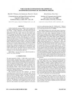
sNB (n′ −D)

xℓ

Estimation of LPC Coefficients

Stat. Model, Codebook

a˜ ℓ

z−D

sNB (n′ )

Feature Extraction

sNB (n) Interpolation

r˜WB (n)

r˜NB (n) Analysis Filter

Residual Signal Extension

Synthesis Filter

s˜WB (n)

Figure 1: Block diagram of the baseline ABWE technique Possible applications of using a-priori known phonetic transcriptions in ABWE training and test are, e.g., offline enhancement of telephone, pilot, or historic speech recordings. Note that Hansen et al. have worked on similar applications for speech enhancement (i.e., noise reduction) that exploits phonetic a-priori knowledge [9]. Another application where time-aligned transcriptions are naturally available is speech synthesis. Here our framework allows for memory efficient speech synthesis corpora, with only NB signals being synthesized and extended in bandwidth in a second step. A further application field of transcription-supported ABWE concerns interactive voice response (IVR) systems in future WB speech networks. Those IVR systems will (of course) exploit the full WB speech in order to allow performancecritical applications, such as dictation or spelling. However, telephone speech databases used to train the acoustic models for automatic speech recognition (ASR) in IVR systems historically consist of NB speech. Since they are phonetically labeled, as is required for ASR training, a telephone speech database extension can be performed in order to save the considerable effort and cost related to recording new telephone speech corpora at higher bandwidth. Last but not least, realtime ABWE employed in conversational telephony can also take profit from phonetic transcriptions. Although the transcription information is certainly not available online, i.e., during ABWE test, we will show that it can be used at least for training purposes to improve the statistical model. Our paper is organized as follows: In section 2 we recapitulate the baseline ABWE approach working on speech waveforms only. Section 3 details a transcription-supported training of ABWE statistical models. Furthermore, a statistical framework is introduced that exploits phonetic transcriptions along with the NB speech waveform during ABWE test. As an application example of the proposed framework, section 4 presents an enhancement of the particularly problematic phoneme class {/s/, /z/}. Experimental results are discussed focusing on the typical lisping and high-frequency whistling effects.

1839

Statistical Model P(sℓ |sℓ−1 ) P(s1 )

Statistical Model

UB Cepstrum Codebook P(sℓ |sℓ−1 ) P(s1 )

(i)

p(xℓ |sℓ )

yˆ UB

UB Cepstrum Codebook P(ϕℓ |sℓ )

p(xℓ |sℓ )

(i)

yˆ UB

xℓ xℓ

P(sℓ |Xℓ )

A-posteriori

UB Envelope

Probabilities ′ φ˜NB (e jΩ )

sNB (n′ −D)

Squared

Assembly of

Periodogram

WB Spectrum

Probabilities

y˜ UB,ℓ

′′ φ˜UB (e jΩ )

P(sℓ |Xℓ , Φℓ ) UB Envelope

A-posteriori

ϕℓ

Estimation

Estimation

′ φ˜NB (e jΩ )

sNB (n′ −D)

Power Spectrum

′′ φ˜UB (e jΩ )

Squared

Assembly of

Periodogram

WB Spectrum

φ˜WB (e jΩ )

y˜ UB,ℓ Power Spectrum

φ˜WB (e jΩ )

Conversion to

Conversion to

LPC Coeffs.

LPC Coeffs.

a˜ ℓ

a˜ ℓ

Figure 2: Baseline estimation of wideband LPC coefficients

Figure 3: Novel estimation of wideband LPC coefficients exploiting phonetic transcriptions ϕℓ

2. THE BASELINE ABWE SYSTEM The high-level baseline ABWE scheme similar to [10] using only the speech waveform is shown in Fig. 1 [11]. It employs a hidden Markov model (HMM) as proposed in [1]. Fig. 2 details the estimation of WB linear predictive coding (LPC) coefficients. A brief overview and some specifics of the system are given now: The narrowband ( fs = 8 kHz) speech signal sNB (n′ ) with sample index n′ is subject to interpolation yielding the upsampled speech signal sNB (n) ( fs = 16 kHz) with sample index n. The actual processing of the interpolated speech signal consists of three steps: A wideband LP (linear prediction) analysis filter, extension of the resulting narrowband residual r˜NB (n) by spectral folding (zeroing every other sample), and final LP synthesis filtering of the extended excitation signal r˜WB (n) using the same coefficients as the analysis filter. Since there are only modifications in the upper frequency band (4 . . . 8 kHz) and the LP analysis and synthesis filters are exactly inverse, this scheme is transparent towards the lower band of the resulting estimated wideband speech signal s˜WB (n). In the following we describe how the estimated wideband LPC coefficient vector a˜ ℓ ∈ R16 in frame ℓ is computed from the narrowband speech signal.

xℓ is computed from a Gaussian mixture model (GMM) obtained in training. Frame-wise state a-posteriori probabilities are then recursively computed by combining the pre-trained state transition probabilities P(sℓ = i|sℓ−1 = j) with the observation PDFs as follows: P(sℓ = i|Xℓ ) = C · p(xℓ |sℓ = i)· N

∑ P(sℓ = i|sℓ−1 = j) · P(sℓ−1 = j|Xℓ−1 ).

(1)

j=1

Note that the sequence of observations is denoted as Xℓ = {xℓ , xℓ−1 , . . . , x1 } and that factor C normalizes the sum of the a-posteriori probabilities over all states sℓ to one. A vector quantizer (VQ) codebook of upper band (UB) (i) cepstral vectors yˆ UB with index i = 1, . . . , N obtained during training is used together with the state a-posteriori probabilities in (1) to perform a minimum mean square error (MMSE) estimation of the upper frequency band in the cepstral domain: N

y˜ UB,ℓ = ∑ yˆ UB · P(sℓ = i|Xℓ ). (i)

(2)

i=1

2.1 Estimation of Wideband LPC Coefficients

′′

After delay compensation to yield a narrowband speech signal sNB (n′ −D) that is time-aligned to its interpolated version at 16 kHz, feature extraction is performed. It operates with a frame length of 20 ms and a frame shift of 10 ms; accordingly the wideband LPC coefficients are updated every 10 ms. The primary features are 10 autocorrelation coefficients, the zero crossing rate, gradient index, normalized relative frame energy, local kurtosis, and spectral centroid, as proposed in [10]. A linear discriminant analysis (LDA) is employed to reduce the dimensionality of the primary feature vector from d0 =15 to d =5. The resulting feature vector xℓ ∈ Rd is subject to a statistical model. Assuming that in frame ℓ the HMM is in a certain state sℓ = i, i ∈ S = {1, . . . , N}, the observation probability density function (PDF) p(xℓ |sℓ = i) for the known observation

This can be converted to the UB power spectrum φ˜UB (e jΩ ) and assembled with the squared periodogram of the lower ′ band φ˜NB (e jΩ ) to the WB power spectrum φ˜WB (e jΩ ). Note that the normalized frequencies Ω′ , Ω′′ cover only the lower and upper band of the wideband signal, respectively. A final conversion via the Levinson-Durbin recursion yields the wideband LPC coefficient vector a˜ ℓ . 2.2 Training Process The training process requires wideband speech data. It is performed offline according to [10] as follows: As a first step, UB cepstral coefficients are derived from each WB speech frame by selective linear prediction (SLP) and subsequent Levinson-Durbin recursion. LBG training then yields the VQ codebook that consists of N cepstral vectors

1840

(i)

yˆ UB = E{yUB |sℓ = i} ∈ R9 representing the upper frequency band. The N codebook entries implicitly define the HMM states sℓ , since each frame ℓ is assigned to a certain index i by vector quantization. In a second step, these classification results are used together with frame-wise obtained primary feature vectors in order to train an LDA matrix as part of the feature extraction in section 2.1. In a third step, state probabilities P(s1 = i) and state transition probabilities P(sℓ = i|sℓ−1 = j) are derived according to [1]. Finally, using the LDA-transformed feature vectors xℓ the parameters of GMM-based observation PDFs p(xℓ |sℓ = i) are trained by means of the expectation maximization (EM) algorithm: A scalar weighting factor, a mean vector, and a diagonal covariance matrix for every d-dimensional normal distribution. For each HMM state, a separately trained GMM of G = 8 mixtures is used. 3. STATISTICAL FRAMEWORK FOR ABWE USING PHONETIC TRANSCRIPTIONS Based on the baseline ABWE system described in section 2, a statistical framework for ABWE exploiting a-priori known phonetic transcriptions along with the speech waveform will be presented in the following. The resulting modifications concerning ABWE training and test are shown in Fig. 3. Note that phonetic transcriptions can be used either within the training process only (section 3.1), or for both training and test (sections 3.1 and 3.2). 3.1 Training Process Using Transcriptions Along with the WB speech signals for training, this section assumes the availability of time-aligned phonetic class labels ϕℓ ∈ P that are taken from the phonetic class alphabet P of size Nϕ ≤ N. Given any HMM state s ∈ S = {1, . . . , N}, these phonetic class labels shall be uniquely related by a mapping function f (s) = ϕ in training. Note that on the other hand, an HMM state s is always uniquely related to an UB cepstral (i) codebook entry yˆ UB with index i, and vice versa, which we denote by s = i. The way the HMM states become phoneme-classspecific in training is that the VQ codebook entries are trained on speech data of a particular phoneme class. This is done by means of supervised training (instead of LBG) (i)

yˆ UB = E{yUB |ϕ = f (s = i)}, i = 1, . . . , N,

(3)

where the given phoneme class ϕ is taken from time-aligned phonetic class labels. Based on a state assignment corresponding to the phoneme-class-specific codebook classes (3), the rest of the training process is performed in analogy to section 2.2, i.e., training of the LDA matrix, of the initial state and state transition probabilities, as well as of the GMM parameters for the observation PDFs. Note that in principle, f (s) = ϕ can be a one-to-one mapping (N = Nϕ ), or multiple states can be assigned to the same phoneme class (N > Nϕ ). In section 4, we will present application experiments to the latter case.

P(sℓ = i|Xℓ , Φℓ ) = C · p(xℓ |sℓ = i) · P(ϕℓ |sℓ = i)· N

∑ P(sℓ = i|sℓ−1 = j) · P(sℓ−1 = j|Xℓ−1 , Φℓ−1 ),

(4)

j=1

with Φℓ = {ϕℓ , ϕℓ−1 , . . . , ϕ1 } being the sequence of transcriptions. Note that here the chain rule has been applied in the form of p(xℓ , ϕℓ |sℓ = i) = p(xℓ |ϕℓ , sℓ = i) · P(ϕℓ |sℓ = i), and due to the tight relation between states and phoneme classes we assumed p(xℓ |ϕℓ , sℓ = i) = p(xℓ |sℓ = i). The term P(ϕℓ |sℓ = i) in (4) denotes the elements of a phonetic transcriptions matrix, which shows that unlike in training, we no longer model the dependency of phoneme class ϕℓ from state sℓ by a unique deterministic function f (sℓ ) = ϕℓ . It expresses the reliability of the transcription process that can be carried out either manually by human transcriptors or automatically by forced Viterbi alignment, and can be modeled by ( 1−ε , if f (sℓ ) = ϕℓ P(ϕℓ |sℓ = i) = (5) ε Nϕ −1 , else, where ε denotes a small value and

∑ P(ϕℓ |sℓ = i) = 1.

ϕℓ ∈P

Please note in (5) the similarity of the (statistically motivated) phonetic transcriptions matrix to the (deterministic) mapping f (sℓ ) = ϕℓ as it was used in training. MMSE estimation of upper band cepstral coefficients is finally performed in analogy to (2) under a moderate interframe smoothing constraint as motivated, e.g., in [12]: q
10 2 · ||y˜ UB,ℓ−1 − y˜ UB,ℓ ||2 ≤ 30 dB. 2 ln10 4. EXPERIMENTS

Investigations about ABWE recently demonstrated that the entries of a speaker-independently LBG-trained VQ codebook obtained from the baseline training process in section 2.2 are insufficient to produce sharp /s/- and /z/-sounds [6]. For these critical phonemes, the LBG-trained codebook entries appear spectrally too flat in the upper frequency band, which is just a consequence of the data in a codebook class being represented by its class mean. This produces lisping effects forming the major obstacle for the acceptance of ABWE. 4.1 Simulation Setup We performed artificial speech bandwidth extension experiments based on the US SpeechDat-Car database [13] in order to investigate the performance on the critical fricative class {/s/, /z/} that was found to be responsible for the typical lisping problem [6]. The required WB speech data for training purposes was taken from six male and six female speakers. Each of them provided two speech sessions. The resulting 24 speech sessions were excluded from the ABWE test. For test purposes a 10% subset of the 404 sessions of the remaining 202 speakers was utilized.

3.2 Estimation of Wideband LPC Coefficients Using Transcriptions

4.1.1 First experiment

The recursive computation of the state a-posteriori probabilities (1) can be modified to exploit phonetic transcriptions by

The first ABWE experiment is just performed according to the baseline scheme of section 2 with N = 24 states.

1841

4.1.2 Second experiment The ABWE test of the second experiment still works according to section 2.1, whereas the training process is already based on section 3.1 making use of phonetic transcriptions. The VQ codebook consists of N = 24 entries that have been trained as follows: We define two phoneme classes. The first phoneme class ϕ = {/s/, /z/} comprises all sounds except phonemes /s/, /z/. It is sufficiently represented by 16 HMM states s ∈ {1, . . . , 16} as shown in [10]. For simplicity, the respective codebook entries are LBG-trained on all available data. The second phoneme class {/s/,/z/} turned out to be sufficiently represented by the remaining 8 HMM states. The training of the 8 codebook entries was found to be advantageously conducted by performing a 64 entry LBG training on /s/ frames only, and keeping only the 8 sharpest centroids. They are determined as those codebook entries with the largest cepstral distance to the mean of the 64 found preliminary centroids, with the important constraint that the 0th cepstral coefficient must be larger than the mean 0th coefficient of the preliminary centroids. These 8 codebook entries are used to commonly represent the fricatives /s/ and /z/ in a sharp fashion. Both can be jointly treated in the upper frequency band, since their discriminating characteristics (voicing properties) are mostly contained in the lower band [6]. 4.1.3 Third experiment The training process of the third experiment is exactly the same as of the second one, however, the ABWE test is performed now according to section 3.2, i.e., also including transcription information. For the statistical framework in (4), the elements of the size 2 × 24 phonetic transcriptions matrix  1 − P(i), if ϕℓ = {/s/, /z/} P(ϕℓ |sℓ = i) = (6) P(i), if ϕℓ = {/s/, /z/} are given by P(i) =



ε, 1 ≤ i ≤ 16 1−ε , 17 ≤ i ≤ 24.

The value ε is assumed as 10−4. Note that this experiment represents a two-class-problem only, i.e., Nϕ = 2 < N = 24. Equation (6) is therefore a simplified variant of (5). 4.2 Experimental Results In order to get a rough impression about the ABWE performance of the three experiments, Fig. 4 exemplarily illustrates the respective spectrograms for the utterance “less poisonous”. Note that the critical fricatives /s/ and /z/ are marked on the top of the figure. The upper graph 4(a) shows the original NB speech spectrogram, whereas the lower graph 4(e) shows the perfect WB speech spectrogram representing the upper bound of performance. As expected, the middle graphs 4(b)-(d) depicting the spectrograms of the three ABWE experiments lie somewhere in between. Note the improvement of 4(c) vs. 4(b) at the first instance of /s/. Apart from that, both spectrograms appear quite similar. A significant improvement can be reported for graph 4(d), which is – for all phoneme instances /s/ and /z/ – very close to graph 4(e). Due to the a-priori known transcription in ABWE training and test, a more precise spectral representation of the upper frequency band is achieved. Hence, the typical lisping effect disappears.

Figure 4: Spectrograms from top to bottom: (a) 8 kHz original speech, (b) baseline ABWE speech (1st experiment) (c) ABWE speech using transcriptions in training only (2nd experiment), (d) ABWE speech using transcriptions in training and test (3rd experiment), (e) 16 kHz original speech; the utterance spoken was “less poisonous”. Fig. 5 shows for all three ABWE experiments time averages of the state a-posteriori probabilities P(sℓ = i|Xℓ ) and P(sℓ = i|Xℓ , Φℓ ), respectively, measured on fricatives. The HMM states sℓ = i of graph 5(b) and 5(c) are phoneme-classspecific according to section 4.1.2 (i.e., including classes 17 to 24 that produce sharp /s/- and /z/-sounds), whereas those of graph 5(a) are not (see section 4.1.1). Nevertheless, there are obviously states in graph 5(a) that clearly represent fricatives, e.g., i = 7, 8, 20 or 23. A serious problem is that these states do not sufficiently discriminate between the two sharpsounding phonemes /s/, /z/ and the other fricatives /S/, /Z/, and /f/. Lisping effects are the consequence. Having a look at graph 5(b), just state sℓ = 4 contributes to the aforementioned lisping problem. In return, a high-frequency whistling artifact is introduced by the additional states i = 17, . . . , 24 that are actually intended for the phoneme class {/s/,/z/}. However, all fricatives more or less contribute to these states, not only /s/ and /z/. Again phonemes /S/, /Z/ and /f/ produce the main confusion: Although they usually exhibit only moderate UB energy, a reconstruction via the last 8 states rather produces a whistling sound. Finally, as expected graph 5(c) reveals a perfect discrimination between the phoneme class {/s/,/z/} (last 8 states) and the other sounds (first 16 states). This significant improvement leads to the reduction of both effects lisping and whistling. 5. CONCLUSIONS We have presented a statistical framework for artificial bandwidth extension (ABWE) that governs the recursive computation of state a-posteriori probabilities exploiting a-priori known phonetic transcriptions along with the narrowband speech waveform. The typical lisping problem of ABWE systems has been reduced by adding {/s/,/z/}-class-specific states through a transcription-supported ABWE training. This already leads to an audible improvement of online ABWE in conversational telephony. However, in some cases slight high-frequency whistling is introduced in return. Therefore, high quality ABWE was presented using phonetic

1842

transcription as a-priori knowledge during training and test. This has been discussed by experimental results and exemplarily confirmed by spectrograms. Informal listening tests revealed a significant improvement of speech quality. Speech samples will be presented at the conference.

P(sℓ = i|Xℓ )

0.6 0.4

6. ACKNOWLEDGEMENTS

0.2

We are thankful to Harald H¨oge from Siemens AG, Munich, Germany, for providing the SpeechDat-Car database in US English. The work was supported by the German Research Foundation (DFG) under grant no. FI 1494/2-1.

0

12 16

sℓ = i

20 24

/s/ /z/ /S/ /Z/ /f/ /v/ /h/ /T/ /D/

REFERENCES

Fri ca

8

tiv es

4

[1] P. Jax and P. Vary, “Wideband Extension of Telephone Speech Using a Hidden Markov Model,” in IEEE Workshop on Speech Coding, Delavan, WI, USA, Sept. 2000, pp. 133–135.

(a) Results of the 1st experiment according to section 4.1.1

[2] J. Kuntio, L. Laaksonen, and P. Alku, “Neural Network-Based Artificial Bandwidth Expansion of Speech,” IEEE Transactions on Audio, Speech and Language Processing, vol. 15, no. 3, pp. 873–881, Mar. 2007. [3] M. L. Seltzer, A. Acero, and J. Droppo, “Robust Bandwidth Extension of Noise-Corrupted Narrowband Speech,” in Proc. of INTERSPEECH, Lisbon, Portugal, Sept. 2005, pp. 1509– 1512.

P(sℓ = i|Xℓ )

0.6 0.4

[4] M. Nilsson and W. B. Kleijn, “Avoiding Over-Estimation in Bandwidth Extension of Telephony Speech,” in Proc. of ICASSP, Salt Lake City, Utah, USA, May 2001, pp. 869–872.

0.2 0 1

24

tiv es

[5] S. Yao and C.-F. Chan, “Block-Based Speech Bandwidth Extension System with Separated Envelope Energy Ratio Estimation,” in Proc. of EUSIPCO, Antalya, Turkey, Sept. 2005. [6] P. Bauer, T. Fingscheidt, and M. Lieb, “Phonetic Analysis and Redesign Perspectives of Artificial Speech Bandwidth Extension,” in Proc. of ESSV, Frankfurt a.M., Germany, Sept. 2008.

Fri ca

1617

sℓ = i

/s/ /z/ /S/ /Z/ /f/ /v/ /h/ /T/ /D/

[7] B. Geiser, P. Jax, and P. Vary, “Robust Wideband Enhancement of Speech by Combined Coding and Artificial Bandwidth Extension,” in Proc. of IWAENC, Eindhoven, The Netherlands, Sept. 2005, pp. 21–24.

P(sℓ = i|Xℓ , Φℓ )

(b) Results of the 2nd experiment according to section 4.1.2

[8] “Speech Codec Speech Processing Functions: AMR Wideband Speech Codec; Transcoding Functions (3GPP TS 26.190, Release 5),” 3GPP; TSG SA, Dec. 2001.

0.6

[9] J. H. L. Hansen and B. L. Pellom, “Text-Directed Speech Enhancement Employing Phone Class Parsing and Feature Map Constrained Vector Quantization,” Speech Communication, pp. 169–190, Apr. 1997.

0.4 0.2

[10] P. Jax, Enhancement of Bandlimited Speech Signals: Algorithms and Theoretical Bounds, Ph.D. thesis, vol. 15 of P. Vary (ed.), Aachener Beitr¨age zu digitalen Nachrichtensystemen, Nov. 2002.

0

24

[11] P. Bauer and T. Fingscheidt, “An HMM-Based Artificial Bandwidth Extension Evaluated by Cross-Language Training and Test,” in Proc. of ICASSP, Las Vegas, NV, USA, Apr. 2008, pp. 4589–4592.

Fri ca

1617

sℓ = i

/s/ /z/ /S/ /Z/ /f/ /v/ /h/ /T/ /D/

tiv es

1

(c) Results of the 3rd experiment according to section 4.1.3

Figure 5: Experimental results: Time-averaged a-posteriori probabilities measured on fricatives in American English

[12] K. Schnell and A. Lacroix, “Time-Varying Linear Prediction for Speech Analysis and Synthesis,” in Proc. of ICASSP, Las Vegas, NV, USA, Apr. 2008, pp. 3941–3944. [13] A. Moreno, B. Lindberg, C. Draxler, G. Richard, K. Choukri, S. Euler, and J. Allen, “SpeechDat-Car: A Large Database for Automotive Environments,” in Proc. of LREC, Athens, Greece, May 2000.

1843