A Stochastic Map For Uncertain Spatial Relationships 1 ... - Core

A Stochastic Map For Uncertain Spatial Relationships Randall Smith Matthew Self Peter Cheeseman SRI International 333 Ravenswood Avenue Menlo Park, California 94025

Abstract In this paper we will describe a representation for spatial relationships which makes explicit their inherent uncertainty. We will show ways to manipulate them to obtain estimates of relationships and associated uncertainties not explicitly given, and show how decisions to sense or act can be made a priori based on those estimates. We will show how new constraint information, usually obtained by measurement, can be used to update the world model of relationships consistently, and in some situations, optimally. The framework we describe relies only on well-known state estimation methods.

1

Introduction

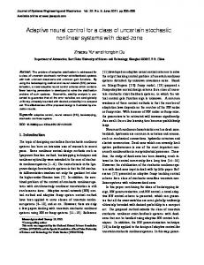
Spatial structure is commonly represented at a low level, in both robotics and computer graphics, as local coordinate frames embedded in objects and the transformations among them — primarily, translations and rotations in two or three dimensions. These representations manifest themselves, for example, in transformation diagrams [Paul 1981]. The structural information is relative in nature; relations must be chained together to compute those not directly given, as illustrated in Figure 1. In the figure the nominal, initial locations of a beacon and a robot are indicated with coordinate frames, and are defined with respect to a fixed reference frame in the room. The actual relationships are x01 and x02 , (with the zero subscript dropped for relations defined with respect to the reference frame). After the robot moves, its relation to the beacon is no longer explicitly described. Generally, nominal information is all that is given about the relations. Thus, errors due to measurement, motion (control), or manufacture cause a disparity between the actual spatial structure and the nominal structure we expect. Strategies (for navigation, or automated assembly of industrial parts) that depend on such complex spatial structures, will fail if they cannot accommodate the errors. By utilizing knowledge about tolerances and device accuracies, more robust strategies can be devised, as will be subsequently shown.

1.1

Compounding and Merging

The spatial structure shown in Figure 1 represents the actual underlying relationships about which we have explicit information. Given a method for combining serial ”chains” of given relationships, we can derive

Figure 1: Robot Navigation: Spatial Structure the implicit ones. If the explicit relationships are not known perfectly, errors will compound in a chain of calculations, and be larger than those in any constituent of the chain. With perfect information, relationship x21 need not be measured — it can be computed through the chain (using x2 and x1 ). However, because of imperfect knowledge, the computed value and the measurement will be different. The difference is resolved by merging the pieces of information into a description at least as ”accurate” as the most accurate piece, no matter how the errors are described. If the merging operation does not do this, there is no point in using it. The real relationships x1 , x2 , and x21 are mutually constrained, and when information about x21 is introduced, the merging operation should improve the

estimates of them all, by amounts proportional to the magnitudes of their initial relative uncertainties. If the merging operation is consistent, one updated relation (vector) can be removed from the loop, as the relation can always be recomputed (by compounding the others). Obviously, a situation may be represented by an arbitrarily complex graph, making the estimation of some relationship, given all the available information, a difficult task.

1.2

Previous Work

Some general methods for incorporating error information in robotics applications([Taylor 1976], [Brooks 1982]) rely on using worst-case bounds on the parameters of individual relationships. However, as worst-case estimates are combined (for example, in the chaining above) the results can become very conservative, limiting their use in decision making. A probabilistic interpretation of the errors can be employed, given some constraints on their size, and the availability of error models. Smith and Cheeseman[Smith, 1984] described six-degree-of-freedom relationships by their mean vectors and covariance matrices, and produced first-order formulae for compounding them. These formulae were subsequently augmented ([Smith, 1985]) with a merging operation — computation of the conditional mean and covariance — to combine two estimates of the same relation. A similar scalar operation is performed by the HILARE mobile robot [Chatila, 1985]. Durrant-Whyte [Durrant-Whyte 1986] takes an approach to the problem similar to Smith and Cheeseman, but propagates errors differentially rather than using the first-order partial derivative matrices of the transformations. Both are concerned with integrating information consistently across an explicitly represented spatial graph. Others [Faugeras 1986],[Bolle and Cooper, 1986] are exploiting similar ideas for the optimal integration of noisy geometric data in order to estimate global parameters (object localization). This paper (amplified in [Smith 1986]) extends our previous work by defining a few simple procedures for representing, manipulating, and making decisions with uncertain spatial information, in the setting of recursive estimation theory.

1.3

The Example

In Figure 1, the initial locations of a beacon and a mobile robot are given with respect to a fixed landmark. Our knowledge of these relations, x1 and x2 , is imprecise, however. In addition, the location of a loading area (the box) is given very accurately with respect to the landmark. Thus, the vector labeled x3 , has been omitted. The robot’s task is to move to the loading area, so that it’s center is within the box. It can then be loaded.

The robot reasons: ”I know where the loading area is, and approximately where I am (in the room). Thus, I know approximately what motion I need to make. Of course, I can’t move perfectly, but I have an idea what my accuracy is. If I move, will I likely reach the loader (with the required accuracy)? If so, then I will move.” ”If not, suppose that I try to sense the beacon. My map shows its approximate location in the room; but of course, I don’t know exactly where I am. Where is it in relation to me? Can I get the beacon in the field of view of my sensor without searching around?” ”Suppose I make the measurement. My sensor is not perfect either, but I know its accuracy. Will the measurement give me enough information so that I can then move to the loader?” Before trying to answer these questions, we first need to create a map, and place in it the initial relations described.

2

The Stochastic Map

In this paper, uncertain spatial relationships will be tied together in a representation called the stochastic map. It contains estimates of the spatial relationships, their uncertainties, and the inter-dependencies of the estimates.

2.1

Representation

A spatial relationship will be represented by the vector of its spatial variables, x. For example, the position and orientation of a mobile robot can be described by its coordinates, x and y, in a two dimensional cartesian reference frame and by its orientation, φ, given as a rotation about the z axis. An uncertain spatial relationship, moreover, can be represented by a probability distribution over its spatial variables. The complete probability distribution is generally not available. For example, most measuring devices provide only a nominal value of the measured relationship, and we can estimate the average error from the sensor specifications. However, the full distribution may be unneccesary for making decisions, such as whether the robot will be able to complete a given task (e.g. passing through a doorway). For these reasons, we choose to model an uncertain spatial relationship by estimating the first two moments of its probability ˆ and the covariance (see Figdistribution—the mean, x ure 2). Figure 2 shows our map with only one object located in it — the beacon. The diagonal elements of the covariance matrix are just the variances of the spatial variables, while the off-diagonal elements are the covariances between the spatial variables. The interpretation of the ellipse in the figure follows in the next section.

2.2

  2 x ˆ σx ˆ=x ˆ 1 =  yˆ  , C(x) =  σxy x σxφ φˆ 

σxy σy2 σyφ

 σxφ σyφ  σφ2

Figure 2: The Map with One Relation Similarly, to model a system of n uncertain spatial relationships, we construct the vector of all the spatial variables, called the system state vector. As before, ˆ , and we will estimate the mean of the state vector, x the system covariance matrix, C(x). In Figure 3 the map structure is defined recursively (described below), providing the method for building it by adding one new relation at at time.









 x  ˆ   , C(x0 ) =  C(x) ˆ0 =  x    ˆn x C(xn , x)

C(x, xn )    C(xn )

Figure 3: Adding A New Object The current system state vector is appended with xn , the vector of spatial variables for a new uncertain relationship being added. Likewise, the current system covariance matrix is augmented with the covariance matrix of the new vector, C(xn ), and its crosscovariance with the new vector C(x, xn ), as shown. The cross-covariance matrix is composed of a column of sub-matrices — the cross-covariances of each of the original relations in the state vector with the new one, C(xi , xn ). These off-diagonal sub-matrices encode the dependencies between the estimates of the different spatial relationships and provide the mechanism for updating all relational estimates that depend on any that are changed. Thus our “map” consists of the current estimate of the mean of the system state vector, which gives the nominal locations of objects in the map with respect to the world reference frame, and the associated system covariance matrix, which gives the uncertainty of each point in the map and the inter-dependencies of these uncertainties. The map can now be constructed with the initial estimates of the means and covariances of the relations x1 and x2 , as shown in Figure 3. If the given estimates are independent of each other, the crosscovariance matrix will be 0.

Interpretation

For some decisions based on uncertain spatial relationships, we must assume a particular distribution that fits the estimated moments. For example, a robot might need to be able to calculate the probability that a certain object will be in its field of view, or the probability that it will succeed in passing through a doorway. ˆ , and covariance matrix, Given only the mean, x C(x), of a multivariate probability distribution, the principle of maximum entropy indicates that the distribution resulting from assuming the least additional information is the normal distribution. Furthermore if the relationship is calculated by combining many different pieces of information, the central limit theorem indicates that the resulting distribution will tend to a normal distribution. We will graph uncertain spatial relationships by plotting contours of constant probability from a normal distribution with the given mean and covariance information. These contours are concentric ellipsoids (ellipses for two dimensions) whose parameters can be calculated from the covariance matrix, C(x) [Nahi, 1976]. It is important to emphasize that we do not assume that the individual uncertain spatial relationships are described by normal distributions. We estimate the first two central moments of their distributions, and use the normal distribution only when we need to calculate specific probability contours. In the figures in this paper, a line represents the actual relation between two objects (located at the endpoints). The actual object locations are known only by the simulator and displayed for our benefit. The robot’s information is shown by the ellipses which are drawn centered on the estimated mean of the relationship and such that they enclose a 99.9% confidence region (about four standard deviations) for the relationships. The mean point itself is not shown. We have defined our map, and loaded it with the given information. In the next two sections we must learn how to read it, and then change it, before discussing the example.

3

Reading the Map

Having seen how we represent uncertain spatial relationships by estimates of the mean and covariance of the system state vector, we now discuss methods for estimating the first two moments of unknown multivariate probability distributions. See [Papoulis, 1965] for detailed justifications of the following topics.

3.1

Uncertain Relationships

The first two moments computed by the formulae below for non-linear relationships on random variables will be first-order estimates of the true values. To

compute the actual values requires knowledge of the complete probability density function of the spatial variables, which will not generally be available in our applications. The usual approach is to approximate the non-linear function y = f (x) by a Taylor series expansion about the estimated ˆ , yielding: mean, x ˆ) + · · · , y = f (ˆ x) + Fx (x − x where Fx is the matrix of partials, or Jacobian, of f ˆ: evaluated at x   ∂f ∂f1 ∂f1 1 · · · ∂x ∂x1 ∂x2 n  ∂f2 ∂f2 ∂f2  · · · ∂x  4 ∂f (x) 4  ∂x1 ∂x 2 n  Fx = (ˆ x) =  . . . .  .. ..  .. ∂x   .. ∂fr ∂fr ∂fr · · · ∂x1 ∂x2 ∂xn x=ˆ x. This terminology is the extension of the fx terminology from scalar calculus to vectors. The Jacobians are always understood to be evaluated at the estimated mean of the input variables. Truncating the expansion for y after the linear term, and taking the expectation produces the linear estimate of the mean of y: ˆ ≈ f (ˆ y x).

(1)

Similarly, the first-order estimate of the covariances are:

C(y) ≈ Fx C(x)FTx , C(y, z) ≈ Fx C(x, z), C(z, y) ≈ C(z, x)FTx .

4

= f (xij , xjk ) = xij ⊕ xjk

xji

= g(xij ) = xij

xjk

= h(xij , xik ) = f (g(xij ), xik ) = xij ⊕ xik

4

4

4

4

4

Utilizing (1), the first-order estimate of the mean of the compounding operation is: ˆ ik ≈ x ˆ ij ⊕ x ˆ jk . x Also, from (2), the first-order estimate of the covariance is:   C(xij ) C(xij , xjk )  JT⊕ . C(xik ) ≈ J⊕  C(xjk , xij ) C(xjk ) where the Jacobian of the compounding operation, J⊕ is given by: 4

(2)

4

xik

J⊕ =

Of course, if the function f is linear, then Fx is a constant matrix, and the first two central moments of the multivariate distribution of y are computed exactly, given correct central moments for x. Further, if x follows a normal distribution, then so does y. In the remainder of this paper we consider only first order estimates, and the symbol “≈” should read as “linear estimate of.”

3.2

we wish to compute the resultant relationship. We denote this binary operation by ⊕, and call it compounding. In another situation, we wish to compute x21 . It can be seen that x2 and x1 are not in the right form for compounding. We must first invert the sense of the vector x2 (producing x20 ). We denote this unary inverse operation , and call it reversal. The composition of reversal and compounding operations used in computing x21 is very common, as it gives the location of one object coordinate frame relative to another, when both are described with a common reference. These three formulae are:

 ∂xik ∂(xij ⊕ xjk ) = = J1⊕ ∂(xij , xjk ) ∂(xij , xjk )

J2⊕

.

The square sub–matrices, J1⊕ and J2⊕ , are the left and right halves of the compounding Jacobian. The first two moments of the reversal function can be estimated similarly, utilizing its Jacobian, J . The formulae for compounding and reversal, and their Jacobians, are given for three degrees–of–freedom in Appendix A. The six degree–of–freedom formulae are given in [Smith 1986]. The mean of the composite relationship, computed by h(), can be estimated by application of the other operations:

Coordinate Frame Relationships

We now consider the spatial operations which are necessary to reduce serial chains of coordinate frame relationships between objects to some resultant (implicit) relationship of interest: compounding, and reversal. A useful composition of these operations is also described. Given two spatial relationships, x2 and x23 , as in Figure 1, with the second described relative to the first,



ˆ jk = x ˆ ji ⊕ x ˆ ik = ˆ ˆ ik x xij ⊕ x The Jacobian can be computed by chain rule as:

J⊕

∂xjk ∂xjk ∂(xji , xik ) = ∂(xij , xik ) ∂(xji , xik ) ∂(xij , xik )     J 0 = J⊕ = J1⊕ J J2⊕ . 0 I 4

=

The chain rule calculation of Jacobians applies to any number of compositions of the basic relations, so that long chains of relationships may be reduced recursively. It may appear that we are calculating firstorder estimates of first-order estimates of ..., but actually this recursive procedure produces precisely the same result as calculating the first-order estimate of the composite relationship. This is in contrast to minmax methods which make conservative estimates at each step and thus produce very conservative estimates of a composite relationship.

sensor update (−)

sensor update

dynamics extrapolation (+)

ˆ k−1 x

ˆ k−1 x -

(−)

(+)

(−)

(+)

ˆk x -

ˆk x -

(−)

(+)

C(xk−1 ) C(xk−1 )

C(xk ) C(xk )

k−1

k

Figure 4: The Changing Map

3.3

Extracting Relationships

We have now developed enough machinery to describe the procedure for estimating the relationships between objects which are in our map. The map contains, by definition, estimates of the locations of objects with respect to the world frame; these relations can be read out of the estimated system mean vector and covariance matrix directly. Other relationships are implicit, and must be extracted, using methods developed in the previous sections. For any relationship on the variables in the map we can write: y = g(x). where the function g() is general (not the function described in the previous section). Conditioned on all the evidence in the map, estimates of the mean and covariance of the relationship are given by: ˆ ≈ g(ˆ y x), C(y) ≈ Gx C(x)GTx .

4

Changing the Map

Our map represents uncertain spatial relationships among objects referenced to a common world frame. It should change if the underlying world itself changes. It should also change if our knowledge changes (even though the world is static). An example of the former case occurs when the location of an object changes; e.g., a mobile robot moves. An example of the latter case occurs when a constraint is imposed on the locations of objects in the map, for example, by measuring some of them with a sensor. To change the map, we must change the two components that define it — the (mean) estimate of the ˆ , and the estimate of the system system state vector, x variance matrix, C(x). Figure 4 shows the changes in the system due to moving objects, and the addition of constraints. A similar description appears in Gelb [Gelb 1984] and we adopt the same notation. We will assume that new constraints are applied at discrete moments, marked by states k. The update of the estimates at state k, based on new information,

is considered to be instantaneous. The estimates, at state k, prior to the integration of the new informa(−) (−) ˆ k and C(xk ), and after the tion are denoted by x (+) (+) ˆ k and C(xk ). At these discrete integration by x moments our knowledge is increased, and uncertainty is reduced. In the interval between states the system may be changing dynamically — for instance, the robot may be moving. When an object moves, we must define a process to extrapolate the estimate of the state vector and uncertainty at state k − 1, to state k to reflect the changing relationships.

4.1

Moving Objects

In our example, only the robot moves, so the process model need only describe its motion. A continuous dynamics model can be developed given a particular robot, formulated as a function of time (see [Gelb, 1984]). However, if the robot only makes sensor observations at discrete times, then a discrete motion approximation is quite adequate. Assume the robot is represented by the Rth relationship in the map. When the robot moves, it changes its relationship, xR , with the world. The robot makes an uncertain relative motion, yR , to reach a final world location x0R . Thus, x0R = xR ⊕ yR . Only a portion of the map needs to be changed due to the change in the robot’s location from state to state — specifically, the Rth element of the estimated mean of the state vector, and the Rth row and column of the estimated variance matrix. In Figure 5, ˆ 0R ≈ x ˆR ⊕ y ˆR, x C(x0R ) ≈ J1⊕ C(xR )JT1⊕ + J2⊕ C(yR )JT2⊕ , C(x0R , xi ) ≈ J1⊕ C(xR , xi ). For simplicity, the formulae presented assume independence of the errors in the relative motion, yR , and the current estimated robot location xR . As in the desciption of Figure 3, C(x, x0R ) is a column of the individual cross-covariance matrices C(xi , x0R ).

The expected value of the sensor value and its covariance are easily estimated as: ˆ ≈ h(ˆ z x). C(z) ≈ Hx C(x)HTx + C(v), 

    0 ˆ = x 0  x  ˆR 



       , C(x0 ) =    C(x0 , x) R    

 C(x, x0R ) C(x0R )

      

Figure 5: The Moving Robot

4.2

Adding Constraints

When new information is obtained relating objects already in the map, the system state vector and variance matrix do not increase in size; i.e., no new elements are introduced. However, the old elements are constrained by the new relation, and their values will be changed. Constraints can arise in a number of ways: • A robot measures the relationship of a known landmark to itself (i.e., estimates of the world locations of robot and landmark already exist). • A geometric relationship, such as colinearity, coplanarity, etc., is given for some set of the object location variables.

where: 4

Hx =

∂hk (x)  (−)  ˆk x ∂x

The formulae describe our best estimate of the sensor’s values under the circumstances, and the likely variation. The actual sensor values returned are usually assumed to be conditionally independent of the state, meaning that the noise is assumed to be independent in each measurement, even when measuring the same relation with the same sensor. The actual sensor values, corrupted by the noise, are the second estimate of the relationship. In Figure 6, an over-constrained system is shown. We have two estimates of the same node, labeled x1 and z. In our example, x1 represents the location of a beacon about which we have prior information, and z represents a second estimate of the beacon location derived from a sensor located on a mobile robot at x2 . We wish to obtain a better estimate of the location of the robot, and perhaps the beacon as well; i.e., ˆ . One method is more accurate values for the vector x to compute the conditional mean and covariance of x given z by the standard statistical formulae: c =x ˆ + C(x, z)C(z)−1 (z − z ˆ) x|z

In the first example the constraint is noisy (because of an imperfect measurement). In the second example, the constraint could be absolute, but could also be given with a tolerance. There is no mathematical distinction between the two cases; we will describe all constraints as if they came from measurements by sensors — real sensors or pseudo-sensors (for geometric constraints), perfect measurement devices or imperfect. When a constraint is introduced, there are two estimates of the geometric relationship in question — our current best estimate of the relation, which can be extracted from the map, and the new sensor information. The two estimates can be compared (in the same reference frame), and together should allow some improved estimate to be formed (as by averaging, for instance). For each sensor, we have a sensor model that describes how the sensor maps the spatial variables in the state vector into sensor variables. Generally, the measurement, z, is described as a function, h, of the state vector, corrupted by mean-zero, additive noise v. The covariance of the noise, C(v), is given as part of the model. z = h(x) + v.

(3)

C(x|z) = C(x) − C(x, z)C(z)−1 C(z, x). Using the formulae in (2), we can substitute expressions in terms of the sensor function and its Jacobian ˆ, C(z), and C(x, z) to obtain the Kalman Filter for z equations [Gelb, 1984] given below: (+)

ˆk x

(−)

ˆk =x

(+)

h i (−) + Kk zk − hk (ˆ xk ) , (−)

(−)

C(xk ) = C(xk ) − Kk Hx C(xk ), h i−1 (−) (−) Kk = C(xk )HTx Hx C(xk )HTx + C(v)k . For linear transformations of Gaussian variables, the matrix H is constant, and the Kalman Filter produces the optimal minimum-variance Bayesian estimate, which is equal to the mean of the a posteriori conditional density function of x, given the prior statistics of x, and the statistics of the measurement z. Since the transformations are linear, the mean and covariances of z are exactly determined by (1) and (2). Since the original random variables were Gaussian, so is he result. Finally, since a Gaussian distribution is completely defined by its first two moments, the conditional mean and covariance computed define the conditional density.

No non-linear estimator can produce estimates with smaller mean-square errors. For example, if there are no angular errors in our coordinate frame relationships, then compounding is linear in the (translational) errors. If only linear constraints are imposed, the map will contain optimal and consistent estimates of the frame relationships. For linear transformations of non-Gaussian variables, the Kalman Filter is not optimal, but produces the optimal linear estimate. The map will again be consistent. A non-linear estimator might be found with better performance, however.







 x  ˆ   , C(x0 ) =  C(x) ˆ0 =  x    ˆ z C(z, x)

 C(x, z)    C(z)

Figure 6: Overconstrained Relationships For non-linear transformations, Jacobians such as H will have to be evaluated (they are not constant matrices). The given formulae then represent the Extended Kalman Filter, a sub-optimal non-linear estimator. It is one of the most widely used non-linear estimators because of its similarity to the optimal linear filter, its simplicity of implementation, and its ability to provide accurate estimates in practice.

5.1

What if I Move?

We combine discrete robot motions by compounding them, as shown in Figure 5. It is assumed that any systematic biases in the robot motion have been removed by calibration. The robot’s best estimate of its ˆ 2 , with error covariance C(x2 ) (given in location is x the map). Since the location of the loading area is known very accurately in room coordinates, the robot can compute the nominal relative motion that it would ˆ 2,load . From an internal model of its like to make, y own accuracy, the robot estimates the covariance of its motion error as C(y2,load ). If there were no errors in the initial estimate of the robot location, and no motion errors incurred in moving, the robot would arrive with its center coincident with the center of the loading area. When the two uncertain relations are compounded, the first-order estimate of the mean of the robot’s final location is also the center of the loading area, but the covariance of the error has increased. In order to compare the likely locations of the robot with the loading zone, we must now assume something about the probability distribution of the robot’s location. For reasons already discussed, a multi-variate Gaussian distribution which fits the estimated moments is assumed. Given that, we can estimate the elliptical region of 2-D space in which the robot should be found, with probability determined by our choice of confidence levels—more than likely corresponding to 4 or 5 standard deviations of the estimated errors, for relative certainty.

The error in the estimation due to the non-linearities in h can be greatly reduced by iteration, using the Iterated Extended Kalman Filter equations [Gelb, 1984]. Such iteration is necessary to maintain consistency in the map when non-linearities become significant. Convergence to the true value of x cannot be guaranteed, in general, for the Extended Kalman Filter, although as noted, the filter has worked well in practice on a large number of problems, including navigation. Figure 7: A Direct Move Might Fail

5

The Example

Our example is designed to illustrate a number of uses of the information kept in the Stochastic Map for decision making. An initial implementation of the techniques described in this paper has been performed. The uncertainties represented by ellipses in the illustrations, were originally computed by the system on a set of sample problems with varying error magnitudes. This description, however, will have to remain qualitative until a more extensive investigation can be performed.

All that remains is to determine if the ellipse is completely contained in the desired region; for purposes of illustration, Figure 7 shows that it is not. The robot decides it cannot achieve its goal reliably by moving directly to the load area.

5.2

Where is the Beacon?

Before moving, the robot can attempt to reduce the uncertainty in its initial location by trying to spot the beacon. The relative location of the beacon to the robot is computed by x2 ⊕ x1 . The two estimated moments of each relation are pulled from the map, and

the moments of the result are estimated, as described in section 3.2. Given the estimate, an elliptical region in which the beacon should be found with high confidence can be computed as before; but this time the relational estimate, and hence the ellipse are described in robot coordinates. The robot can compare this region with the region swept out by the field of view of its sensor to determine if sensing is feasible (without repositioning the sensor, or worse, turning the robot). The result is illustrated in Figure 8.

ˆ 2 and Hx , and is evaluated with the current values of x ˆ 1 , the robot and beacon locations. The updated sysx tem covariance matrix can be computed as if the sensor were used. The reduction in the robot’s locational uncertainty due to applying the sensor can be judged by comparing the old value of C(x2 ) with the updated value. The magnitudes of this ”updated” robot covariance estimate, and C(y2,load ) (from 5.1), can be used to decide if the robot will be able to reach its goal with the desired tolerance.

The robot determines that the beacon is highly likely to be in its field of view.

Figure 9: The Robot Senses the Beacon Again

Figure 8: Is the Beacon Viewable?

5.3

Should I Use the Sensor?

Even if the robot sights the beacon, will the additional information help it estimate its location accurately enough so that it can then move to the loader successfully? If not, the robot should pursue a different strategy to reduce its uncertainty. For simplicity, we assume that the robot’s sensor measures the relative location of the beacon in Cartesian coordinates. Thus the sensor function is the functional composition of reversal and compounding, already described. The sensor produces a measurement with additive, mean-zero noise v, whose covariance is given in the sensor model as C(v). Given the information in the map, the conditional mean and covariance of the expected sensor value can be estimated:

Figure 10: Updated and Original Estimates

z = x21 = x2 ⊕ x1 . ˆ=x ˆ 21 = ˆ ˆ1. z x2 ⊕ x  C(z) = J⊕

C(x2 ) C(x2 , x1 ) C(x1 , x2 ) C(x1 )



T J⊕

+ C(v).

In the Kalman Filter Update equations described in section 4.2, the system covariance matrix can be updated without an actual sensor measurement having been made; it depends only on C(x), C(v), and the matrix Hx . In the example, J⊕ takes the place of

Figure 11: The Robot Moves Successfully In our example, it is determined that the sensor should be useful. Figure 9 shows the result of a simulated measurement, with the location and measure-

ment uncertainties transformed into either robot or map coordinates, respectively. Figure 10 illustrates the improvement in the estimations of the robot and beacon locations following application of the Kalman Filter Update formulae with the given measurement. Finally, Figure 11 shows the result of compounding the uncertain relative motion of the robot with its newly estimated initial location. The robot achieves its goal.

Although the examples presented in this paper have been solely concerned with spatial information, there is nothing in the theory that imposes this restriction. Provided that functions are given which describe the relationships among the components to be estimated, those components could be forces, velocities, time intervals, or other quantities in robotic and non-robotic applications.

6

Appendix A: Three DOF Relations

Discussion and Conclusions

This paper presents a general method for estimating uncertain relative spatial relationships between reference frames in a network of uncertain spatial relationships. Such networks arise, for example, in industrial robotics and navigation for mobile robots, because the system is given spatial information in the form of sensed relationships, prior constraints, relative motions, and so on. The methods presented in this paper allow the efficient estimation of these uncertain spatial relations and can can be used, for example, to compute in advance whether a proposed sequence of actions (each with known uncertainty) is likely to fail due to too much accumulated uncertainty; whether a proposed sensor observation will reduce the uncertainty to a tolerable level; whether a sensor result is so unlikely given its expected value and its prior probability of failure that it should be ignored, and so on. This paper applies state estimation theory to the problem of estimating parameters of an entire spatial configuration of objects, with the ability to transform estimates into any frame of interest. The estimation procedure makes a number of assumptions that are normally met in practice, and can be summarized as follows: • Functions of the random variables are relatively smooth about the estimated means of the variables within an interval on the order of one standard deviation. In the current context, this generally means that angular errors are “small”. In Monte Carlo simulations[Smith, 1985], the compounding formulae were used on relations with angular errors having standard deviations as large as 5o , gave estimates of the means and variances to within 1% of the correct values. Wang [Wang] analytically verified the utility of the first-order compounding formulae as an estimator, and described the limits of applicability. • Estimating only two moments of the probability density functions of the uncertain spatial relationships is adequate for decision making. We believe that this is the case since we will most often model a sensor observation by a mean and variance, and the relationships which result from combining many pieces of information become rapidly Gaussian, and thus are accurately modelled by only two moments.

Formulae for the full 6DOF case are given in [Smith 1986]. The formulae for the compounding operation are: xik

4

= xij ⊕ xjk   xjk cos φij − yjk sin φij + xij =  xjk sin φij + yjk cos φij + yij  . φij + φjk

where the Jacobian for the compounding operation, J⊕ is: 4

J⊕ =



1  0 0

∂xik ∂(xij ⊕ xjk ) = = ∂(xij , xjk ) ∂(xij , xjk )

0 −(yik − yij ) 1 (xik − xij ) 0 1

cos φij sin φij 0

− sin φij cos φij 0

 0 0 . 1

The formulae for the reverse operation are:   −xij cos φij − yij sin φij 4 4 xji = xij =  xij sin φij − yij cos φij  . −φij and the Jacobian for the reversal operation, J is:  − cos φij ∂x 4 ji J = =  sin φij ∂xij 0

− sin φij − cos φij 0

 yji −xji  . −1

References Bolle R.M., and Cooper, D.B. 1986. On Optimally Combining Pieces of Information, with Application to Estimating 3-D Complex–Object Position from Range Data. IEEE Trans. Pattern Anal. Machine Intell., vol. PAMI-8, pp. 619-638, Sept. 1986. Brooks, R. A. 1982. Symbolic Error Analysis and Robot Planning. Int. J. Robotics Res. 1(4):29-68. Chatila, R. and Laumond, J-P. 1985. Position Referencing and Consistent World Modeling for Mobile Robots. Proc. IEEE Int. Conf. Robotics and Automation. St. Louis: IEEE, pp. 138-145.

Durrant–Whyte, H. F. 1986. Consistent Integration and Propagation of Disparate Sensor Observations. Proc. IEEE Int. Conf. Robotics and Automation. San Francisco: IEEE, pp. 1464-1469. Faugeras, O. D., and Hebert, M. 1986. The Representation, Recognition, and Locating of 3-D Objects. Int. J. Robotics Res. 5(3):27-52. Gelb, A. 1984. Applied Optimal Estimation. M.I.T. Press Nahi, N. E. 1976. Estimation Theory and Applications. New York: R.E. Krieger. Papoulis, A. 1965. Probability, Random Variables, and Stochastic Processes. McGraw-Hill. Paul, R. P. 1981. Robot Manipulators: Mathematics, Programming and Control. Cambridge: MIT Press. Smith, R. C., et al. 1984. Test-Bed for Programmable Automation Research. Final Report-Phase 1, SRI International, April 1984. Smith, R. C., and Cheeseman, P. 1985. On the Representation and Estimation of Spatial Uncertainty. SRI Robotics Lab. Tech. Paper, and Int. J. Robotics Res. 5(4): Winter 1987. Smith, R. C., Self, M., and Cheeseman, P. 1986. Estimating Uncertain Spatial Relationships in Robotics. Proc. Second Workshop on Uncertainty in Artificial Intell., Philadelphia, AAAI, August 1986. To appear revised in Vol. 2, Uncertainty in Artificial Intelligence. Amsterdam: North–Holland, Summer 1987. Taylor, R. H. 1976. A Synthesis of Manipulator Control Programs from Task-Level Specifications. AIM282. Stanford, Calif.: Stanford University Artificial Intelligence Laboratory. Wang, C. M. 1986. Error Analysis of Spatial Representation and Estimation of Mobile Robots. General Motors Research Laboratories Publication GMR 5573. Warren, Mich.