Key words, dynamic storage allocation, checkerboarding, M/M/o queue, memory allocation. 1. Introduction. Adopting the terminology ofqueues, suppose ...
SIAM J. COMPUT. Vol. 14, No. 2, May 1985
1985 Society for Industrial and Applied Mathematics 012
A STOCHASTIC MODEL OF FRAGMENTATION IN DYNAMIC STORAGE ALLOCATION* E. G. COFFMAN, JR.’, T. T. KADOTAf
AND
L. A. SHEPPf
Abstract. We study a model of dynamic storage allocation in which requests for single units of memory arrive in a Poisson stream at rate A and are accommodated by the first available location found in a linear scan of memory. Immediately after this first-fit assignment, an occupied location commences an exponential delay with rate parameter/z, after which the location again becomes available. The set of occupied locations (identified by their numbers) at time forms a random subset S, of 1, 2, .}. The extent of the fragmentation in S,, i.e. the alternating holes and occupied regions of memory, is measured by max (St) -IStl. In equilibrium, the number of occupied locations, ISI, is known to be Poisson distributed with mean p A//x. We obtain an explicit formula for the stationary distribution of max (S), the last occupied location, and by independent Moreover, we verify arguments we show that (E max (S) EISI)/EISI- 0 as the traffic intensity /9 numerically that for any/9 the expected number of wasted locations in equilibrium is never more than 1/2 the expected number of occupied locations. Our model applies to studies of fragmentation in paged computer systems, and to containerization problems in industrial storage applications. Finally, our model can be regarded as a simple concrete model of interacting particles [Adv. Math., 5(1970), pp. 246-290].
.
Key words, dynamic storage allocation, checkerboarding, M/M/o queue, memory allocation
1. Introduction. Adopting the terminology of queues, suppose customers arrive in a Poisson stream at rate A to a linear queue of waiting or storage locations numbered 1, 2,.... According to the so-called first-fit policy each customer occupies the lowest numbered location available at his time of arrival. Immediately upon being installed in an available location, a customer commences a delay or residence time having an exponential distribution with parameter/x. At the end of his residence time a customer departs from the queue, thus making available the location he occupied. As locations are occupied and released "holes" build up, so that the total occupancy, defined as the highest numbered location occupied by waiting customers, may be substantially greater than the number of customers in the queue. The principal objectives of this paper are an analysis leading to the stationary distribution of this total occupancy, and a characterization of the fraction of wasted space under heavy-traffic conditions, i.e. for
large In queueing parlance our model may be recognized as an M/M/c queue on which a first-fit discipline for placement into a linear sequence of servers has been superimposed. The equilibrium distribution for the number in system is well-known for the M/M/ system [4, p. 414]. Although we shall make some use of these classical results, we focus on the more difficult analysis of the total occupancy process, an analysis that is clearly more important in the applications noted below. Similar results for an M/M queue have been obtained in [2], where conventional methods were found to be adequate. The greater difficulty of our problem stems from the more easily motivated, but combinatorially more complex, first-fit placement rule. Interpreting customers as requests for single units of storage, our model is an instance of the general problem of dynamic storage allocation in computers. The elements of this subject have been treated by Knuth [6], and a recent survey appears in ]. In particular, the infinite-server model was introduced in [6, p. 445] in an analysis of the well-known fifty-percent rule.
"
Received by the editors September 28, 1982, and in revised form January 30, 1984. AT&T Bell Laboratories, Murray Hill, New Jersey 07974.
416
417
STOCHASTIC MODEL OF FRAGMENTATION
Paged computer systems are specific applications of our model. Here, single units of storage become pages and locations become page frames, i.e. sets of consecutive memory locations that can accommodate exactly one page and that begin at integral multiples of the fixed page size. As before, the analysis of total occupancy leads to a characterization of the extent of fragmentation that occurs as pages come and go under a first-fit rule. Indeed, by an appropriate substitution of terms, our model applies quite generally to any such first-fit storage/server assignment problem where locations would correspond, for example, to telephone trunks, parking spaces, etc. There are a number of extensions to our model which would broaden its applicability. These, along with their implications for the analysis of stochastic models, are discussed in the last section. Our analysis starts with the observation that the total occupancy process cannot be formulated as a Markov chain. We then identify a bivariate Markov chain in continuous time from which the stationary state probabilities of this process can be calculated. This calculation amounts primarily to a solution of the partial differential equation governing the generating function for the equilibrium probabilities of the bivariate Markov chain. For this purpose we adopt an apparently novel approach with generating functions, whereby a partial differential equation is replaced by an infinite but solvable system of ordinary differential equations. By an independent argument bounds on the expected total occupancy are derived; asymptotic properties of the total occupancy process are deduced from these bounds. In the next section the mathematical model is formally defined. The major results, 3 and 4. also presented in the next section, are then proved in 2. Mathematical model. For a fixed traffic intensity p A//x > 0 consider a continuous time Markov chain Mo whose states are the (finite) subsets of {1, 2,...}. A given state St is just that collection of numbers corresponding to occupied locations at time t. Transitions occur at rate /x > 0 from any nonempty S to each of the sI subsets of S obtained by deleting one location from S, and at rate A from any S to the union of S and the smallest numbered location not in S. Because S diminishes at rate [SI/x, it is easy to see that for any p, if ISol < then ISt[ < for all t> 0 with probability and that Mp is a Markov chain with a stationary distribution on the set of finite subsets of {1, 2,...}. It does not seem possible to obtain the stationary distribution of S, but we are able to find this distribution for both IsI and max (S), the maximum element of S. Note that max (S) is simply the total occupancy mentioned in the previous section. denote the stationary distribution, we Letting ’71"k limt.P(lStl k), k 0, 1, have the following standard results from the analysis of an M/M/ queue [4]
,
k
(2.1)
7rk
=.
k=0, 1,...
e
and
E lSl
(2.2)
(2.3)
Y.
p.
k>_O
Next, consider the distribution of max (S). We will prove in 3 that (-1) m-0, 1,...o P(max (S)> m) 2 ,=o
n+l
k=O
-,
Note that for m=0, P(max (S)>0)= I-P(S=)= l-P(ISl=0) l-e as seen from (2.1), and (2.3) agrees with this result. For m 1, the right side of (2.3) becomes
418
E. G. COFFMAN, JR., T. T. KADOTA AND L. A. SHEPP
an integral and
P(max (S) > 1)
e --pxl/’ dx.
However, for large m and p, calculation of the right side of (2.3) is awkward. For these cases we can make use of the following crude bounds, trm -- m) _=ISI so that P(max (S)> m)>=P([Sl> m); the first inequality thus follows from (2.1) and (2.5). For the second, note first that
(2.6) P(max (S)> m) m) m). m=K
m=O
Choosing K
(2.9)
[(1+ e)pJ and using (2.4) and (2.8), we have, since tr,’l, E max (S) 0, 1- crK_l--> 0 as p-> oo, [4, p. 193] it follows from (2.9) that
(2.10)
lim
E max (S) -- ISI,.thus E max (S)_>-EIS
(2.11)
E(max(S)-ISI)=o(EISI)
p. Hence
as p.
Thus, as p
the wastage becomes negligible relative to the number of occupied locations. The method of (2.8) can be used to tighten the bound of (2.9) on E max (S) by applying (2.8) for K [(p log p)/J instead of K [(1 + e)pJ. In fact we show in 4 that
(2.12)
E(max (S)-[SI) --< c(p log p)/=
for some constant c. For an even closer look at asymptotic behavior numerical calculations were worked out by using (2.3) directly in (2.8). A plot of log P(max (S)> m)
419
STOCHASTIC MODEL OF FRAGMENTATION
vs. log 1/p revealed a nearly linear graph and thus indicated that, as p-
E(max(S)-ISl)--,c’p ’,
(2.13)
for constants a and c’. The numerical results showed that a -0.42. In Fig. l, the wastage rate, defined as (E max (S)-EISI)/EISI, is plotted as a function of 1/EISI 1/p. It shows that the wastage rate approaches 0 monotonically as p--> oo and p--> 0. What is more interesting, however, is the existence of a maximum clearly less than 1/3 at lip- 0.40 and the strictly monotone behavior on both sides of the maximum. Thus, E max (S) is at most times E[S I. Q55
0.:30
0.25
0.20
0:15
0.40
0.05
" ]1
0.0
2
5
5
4
6
7
8
9
’10
1/p(=l/ElSl) FIG. 1.
3. Derivation of (2.3). The derivation depends first on the use of an embedded two-dimensional Markov process and then on the use of a novel technique with generating functions. The embedded Markov process is (IStf]{1,2,..., m}l IStfq { m + l, m + 2, .}]) which is Markovian on states of integer pairs (k, r), 0 _-< k -l.
421
STOCHASTIC MODEL OF FRAGMENTATION
Rewriting (3.14),
(3.15) /)(1)
due-U(u-1)num=
fn-)(1)
due-U(u 1)n-lu m,
i---i’i
n>= 1,
we observe that the function described by the left side of (3.15) does not depend on n =0, 1,2,.... Setting n in the right side of (3.15), then using (3.10) and the fact that F(1, 1)= 1, we have
f’(1
due_O,(u_l),u nt Now, using Taylor’s expansion about y 1,
(3.16)
(3.17)
f(Y)=
E
f)(1)
due_OUu___
01
p
f)(1)(y-1) n!
.=o
Since the coefficients w(m, r) in (3.6) satisfy (m, r)P([SI m+ r)= O(1/rt) by (2.1), f is an entire function and the validity of (3.17) follows. Using (3.16) and (3.17), we have e
-
f(Y)=
(3.18)
Then, from (3.8),
(3.19)
E
O n=o
F(1, y)
e
-
(Y- 1)"
E
,=o
I
du e-"(u
(y 1)"+’ (n+ 1)
,
1)"U
du e-"(u- 1)nu
and setting y =0 gives (2.3) because of (3.7). We obsee finally that the joint distribution of max (S) and ISI can be obtained from F(x, y), which is determined from (3.13) and (3.16) explicitly. Indeed
(3.20)
P(max (S) m, ISI
2 (J, 0; m)
k)
j=O
and w(L 0; m)=(L O)=g/OxF(O,O), which can be obtained from F(x,y). The resulting expression for the joint distribution of max (S) and SI does not appear to have a simple form and is therefore omitted. 4. Derivation of (2.12). First, note that
(4.1)
= m!- K
1+
+
+
x>O.
K K-x’
From (2.8) and (2.4) with p x
(4.2)
x
E max(S)K+x m=K
as xSince e -vt =o (x/J t) (4.1) with Stirling’s formula,
E max (S)
(4.3)
m Ejo (x/J)"
[4, p 193], by setting K
x + y + ClX e
X
x+y
[x+yJ we obtain, using X
+y
(x + y)/(x + y)+Y e -*+y) y Cl(X + y)3/2ey