A Strategy for Constructing Models to Minimize Prediction Uncertainty Randall J. Hunt1, John Doherty2 U.S. Geological Survey,
[email protected], Middleton, WI, USA 2 Watermark Numerical Computing,
[email protected], Corinda, Australia 1
ABSTRACT Models are a simplification of reality, but all the parameters that relate a stress to system response need to be included to accurately predict the response to a future stress. Some parameters important to prediction accuracy may be lost in the simplification process. At the same time funding constraints make it difficult to decide how efforts should be divided between model construction and the collection of additional data. Modeling reports commonly conclude with a desire for more data and calibration; how well the model can simulate future stress, and how worthwhile the modeling effort is to decision makers, is often uncertain. To address these issues, a strategy for constructing models is proposed that uses regularized inversion and single-value decomposition. Using this approach, initial parameter complexity more closely reflects the underlying detail of the system and uncaptured detail is minimized. Moreover, model parsimony is employed automatically through single-value decomposition process resulting in a more stable and well-posed parameter estimation. In addition to non-linear regression benefits, the approach proposed can be used for a pre-calibration analysis that identifies: 1) parameters important for a prediction of interest; 2) an estimate of the commonly uncharacterized model structure error; and 3) the amount of parameterization needed to minimize the total prediction uncertainty. A case study using a steady-state model of the USGS Trout Lake Water, Energy and Biogeochemical Budgets (WEBB) site in northern Wisconsin is presented to illustrate the approach. INTRODUCTION Model structure introduces simplifications to reality in the form of layering and parameter and boundary condition zones. Simplification inherent to model structure is itself a source of uncertainty in any application of the model, and often introduces more uncertainty than does the uncertainty associated with noise in the observations used to calibrate the model (Moore and Doherty 2005). However, structural uncertainty is routinely neglected when evaluating possible prediction error. In practice, calibration is often considered the primary action for reducing prediction uncertainty, and new calibration methods (pilot-points – Doherty 2003; regularization and parameter subspace methods – Tonkin and Doherty 2005) have allowed us to characterize how much parameter heterogeneity the model should contain given available data and geologic knowledge. Commonly collected calibration data, however, may not provide sufficient information to constrain parameters important for model prediction (e.g., Kelson et al. 2002). In a model of the Trout Lake watershed in Wisconsin, several types of data have been collected that are potentially useful in model calibration, including commonly collected head and flux data. Less commonly collected data available for this basin include water isotopes, strontium isotopes, calcium concentrations, and groundwater age dating. This range of calibration data types provides a good test for how calibration data can and cannot improve model predictions. In this paper, we describe how the approach of Moore and Doherty (2005) can improve the accuracy of predictions obtained using a watershed-scale flow model. STRATEGY TO MINIMIZE PREDICTION UNCERTAINTY The strategy that we propose here is consistent with the idea of “stepwise modeling” (Haitjema 1995). The idea is that problems can be first modeled with existing data and then results from initial modeling can be used to guide future modeling and data collection. Specifically, we propose that: 1) an initial model be constructed and highly parameterized; 2) estimates of variance around model parameters be made before calibration; 3) single-value decomposition (SVD -Tonkin and Doherty 2005) be used to quantify prediction uncertainty; 4) benefits of calibration and the future data collection be formally evaluated. Of these, we’ll focus on the pre-calibration analysis and calculation of prediction uncertainty.
Prediction uncertainty and pre-calibration analysis: Analysis of the error variance of critical predictions undertaken by the model can be implemented using methods described in Moore and Doherty (2005). This work demonstrates that prediction uncertainty springs from two components: 1) Effects of Measurement Noise: Exact estimation of appropriate parameter values is not possible due to measurement noise. Thus uncertainty in predictions which depend on these parameter combinations can never be eliminated – only reduced. This is the only component considered in traditional calculations of error variance. 2) Failure to Capture Real-World Heterogeneity: This component represents the contribution of uncaptured parameterization (i.e., the “calibration null space”) to model predictive uncertainty. This represents artifacts from errors in model structure (thus heterogeneity that is beyond the ability of the calibration process to capture) and is often the dominant contributor, especially for those predictions that are sensitive to system detail. Where a prediction depends on system detail (for example transport problems), the neglect of the second component can lead to considerable errors. Cooley (2004) describes a method for quantifying the structural component of prediction error involving many model runs for a given model structure. As an alternative, Moore and Doherty (2005) suggest that both components of error variance can be calculated employing matrices that are produced as an outcome of regularised inversion. Moreover, the application of the Moore and Doherty (2005) approach does not require that the model actually be calibrated; all that is required are sensitivities of model-generated observation equivalents to parameters and a relation of key predictions to parameters. Therefore, using a notional SVD calibration exercise based on scaled parameters, one can determine:
Pre-calibration predictive error variance The number of singular values required for the forthcoming calibration exercise in order to minimize predictive error variance The contribution that different parameters and boundary conditions will make to predictive error variance. The contribution that certain existing or posited observations will make to reducing error variance.
Because such an analysis includes the important null-space component it is a more accurate indicator of true prediction error than statistics which ignore it. An analysis such as the above can provide considerable assistance in determining what data to gather, and even whether the calibration process is worthwhile. It can also assist in determining whether holding certain parameters and boundary conditions constant during the forthcoming calibration process is likely to incur predictive error. Approach for calculating prediction uncertainty: Post calibration computation of predictive error variance can be undertaken using the formula of Moore and Doherty (2005) applying matrices derived from the calibration process. Nonlinear predictive error variance analysis can also be undertaken using an extension of the method of Vecchia and Cooley (1987) where a limiting objective function is formulated on the basis of model-to-measurement misfit (applied to the parameter solution space) and parameter reasonableness (applied to the parameter null space). Either of these analyses allows full quantification of predictive error taking into consideration both the null space structural component and measurement noise component. Software for implementation of such analyses is available through the PEST suite. SITE DESCRIPTION AND PREVIOUS MODELING The Trout Lake basin is located in the Northern Highlands district in north central Wisconsin, in an area with many lakes (Figure 1). The aquifer consists of 40-60 m of unconsolidated Pleistocene glacial sediments mostly consisting of glacial outwash sands and gravel. The Trout Lake basin (which includes Trout Lake and all four of the basins that flow into the lake) has been the focus of previous regional modeling studies including a two-dimensional analytic element screening model and three-dimensional, finite-difference models. See Pint (2002) and Hunt et al. (2005) for more description of the setting and previous modeling.
MODELING APPROACH Model Construction: A three-dimensional model using MODFLOW2000 was constructed for the 310 square kilometer area that includes the greater Trout Lake basin (Pint 2002). The model included areas outside the Trout Lake basin to allow groundwater divides to move as the model was calibrated. This is important here because the groundwatershed and surface watershed are not aligned and the groundwatershed is estimated to be >40% larger than the surface watershed. Thirty lakes within the Trout Lake basin or near its boundary were simulated using the LAK3 Lake Package. Streams that are located within the Trout Lake basin were simulated using the Streamflow Routing Package. All other lakes and streams were represented using the River Package. Figure 1. Location of pilot points (crosses), near-field lakes (dark), near-field streams (dark), far-field lakes (light), and far-field rivers (light). Crystal Lake, used for the prediction analysis is also shown. The Trout Lake WEBB model was calibrated using the parameter estimation code PEST (Doherty, 2005) using pilot points (Doherty 2003) (Figure 1), and regularization assisted singlevalue decomposition (SVD-Assist). This approach allowed estimation of over 950 parameters compared to the maximum 11 parameters using Crystal previous approaches described by Hunt et al. Lake (2005). The majority of the parameters were pilot points for estimating horizontal and vertical hydraulic conductivity in each layer; in addition, three recharge zones, two porosity zones and 43 lakebed leakance zones were also allowed to vary during model calibrations. Other parameters (Manning’s roughness, near-field stream stage, far-field river stage) and parameterization schemes (pilot points for recharge) were evaluated in initial calibration runs but found to not be important for the prediction types of interest. Five types of targets were used. The first two, water levels from lakes and wells and base flow targets, are typically used in groundwater models. Groundwater level measurements from 58 wells measured from a near average period (July 2001) were used as head targets. The 10-year median base flow values for four streamflow targets were used as flux targets. As discussed by Hunt et al. (2005), three types of unconventional data were also used in the parameter estimation objective function, and included: 1) groundwater fluxes to and from 11 selected lakes in the basin obtained using a stable-isotope mass balance and water budget analysis; 2) elevation of the top of a Big Musky Lake plume at two locations in the aquifer as identified in a nested piezometer shown in these locations using water isotopes; 3) time of travel to two well nests estimated using CFC and tritium sampling. RESULTS AND DISCUSSION Pre- and post-calibration analysis: For brevity, the discussion will focus on a single prediction of change in Crystal Lake stage (figure 1) in response to a drought scenario (10% reduction in precipitation, 10% increase in lake evaporation). Given the model structure and an estimate of the variance around each parameter prior to calibration, the uncalibrated model can be expected to calculate the present stage with a prediction variance of about 0.7 m, or a standard deviation of about 0.8 m (shown by the intersection of the solid black line with the y-axis in Figure 2). The uncalibrated model can be expected to estimate the lake stage under drought conditions with a variance of about 1 m (shown by the intersection of the black dotted line and the y-axis), and is consistent with a larger error variance expected for a relatively more unknown future condition. If this level of accuracy was sufficient (say, in a scoping calculation) the modeler may choose to stop there and not calibrate the model. Note that if the structural
Predictive Error Variance (m2)
or null space component of uncertainty was ignored and only measurement noise was considered, the expected error of the prediction would be near zero for both the present day and drought condition.
Crystal Lake Stage – Calibration and Prediction (drought conditions)
4
Figure 2. Prediction error variance versus parameterization for a prediction of Crystal Lake stage under present day and drought conditions. Both the traditional measurement error component and commonly ignored structural or “null space” error are shown. The black lines reflect the total prediction uncertainty calculated by summing the two components.
total error
3
2 measurement noise error
drought prediction (dashed)
Calibration can reduce the predictive error variance as demonstrated by the reduction of total prediction 1 uncertainty as the number of parameters increases to about 25 or 30 (figure 2). This indicates that the model structural error existing calibration data do contain information that can constrain the model calibration for the purposes calibration (solid) of this prediction. There is a tradeoff, however, 0 between the reduction in structural error provided by 0 40 80 120 increased parameterization and the decreased Dimensionality of Inverse Problem ability of the observations to constrain the parameters (as shown by the increasing (# of parameters) measurement noise component at higher parameterization). Thus, for this particular prediction and model structure, 25 to 30 parameters seem to provide the least amount of prediction uncertainty. This is appreciably greater than the maximum of 11 parameters estimated by Pint (2002) and Hunt et al. (2005). Furthermore, we expect that the prediction error variance could be further reduced if additional flexibility was included in the model construction (e.g., more layers). As might be expected, the contribution to the prediction uncertainty was not uniform for all parameter types (figure 3), which underscores the prediction-specific nature of the insight. Moreover, the reduction in prediction error variance due to calibration was also not uniform, demonstrating that information contained in the existing calibration data can constrain some parameters for the purposes of this prediction better than others. For example, the calibration data did 0.30 not appreciably change the 0.20 0.15 0.10 0.05
post-calibration
kz4
kz3
kz1
kz2
k3
k4
k1
pre-calibration
k2
inc rchg
0.00 man por lk leakance rstage
variance
(m2)
0.25
Figure 3. Pre- and postcalibration contribution to prediction uncertainty for parameter types used in the model (man=Manning’s n, por=porosity, lk leakance =lakebed leakance, rstage=farfield river stage, inc=stream elevation increment, rchg= recharge, k1 through k4-=Kh of layers 1 through 4, kz1 through kz4=Kz of layers 1 through 4).
contribution from the horizontal and vertical hydraulic conductivity of layer 1 (figure 3). The horizontal hydraulic conductivity of layers 3 and 4, on the other hand, were appreciably improved during calibration and, as a consequence, contributed less to the prediction uncertainty. As shown by Hunt et al. (2005), diverse data types can enhance model calibration. These data can also be important for reducing prediction uncertainty (figure 3). Of the parameters tested, the largest reduction to the prediction variance from calibration occurred due to a decrease in the prediction variance associated with lakebed leakance (vertical arrow in figure 3). Leakance is often difficult to constrain with head or streamflow field data (Hunt 2002; Kelson et al. 2002); observations of groundwater inflow into the lake, as calculated by a stable isotope mass balance approach, do constrain lakebed leakance however (Hunt et al. 2005). Thus, using models to evaluate the utility of “diverse” data can facilitate cost-benefit analyses for future data collection. Finally, it is apparent that future data collection can be targeted to reduce the uncertainty around this prediction. Clearly, additional knowledge of some parameters (porosity, Manning’s n, lakebed leakance, vertical conductivity of layers 3 and 4) will not lead to more a more accurate prediction of lake stage under drought (Figure 3). Indeed, in the case of lakebed leakance, not much is gained from future characterization after the model is calibrated. Rather, a data collection effort targeted at the horizontal conductivity of the lower part of the aquifer (layers 3 and 4), and to a lesser extent layer 1, will do most for reducing the uncertainty around this prediction. ACKNOWLEDGEMENTS This work was funded by the U.S. Geological Survey’s Trout Lake Water, Energy, and Biogeochemical Budgets (WEBB) program, in cooperation with NSF’s North Temperate Lakes LTER program (DEB9632853). REFERENCES Cooley, R.L., 2004. A theory for modeling ground-water flow in heterogeneous media: U.S. Geological Survey Professional Paper 1679, 220 p. Doherty, J., 2003. Groundwater model calibration using pilot points and regularization, Ground Water 41(2), 170-177. Doherty, J., 2005. Manual for PEST: Model-Independent Parameter Estimation. Fifth Edition. Watermark Numerical Computing, Brisbane, Australia Haitjema, H.M., 1995. Analytic Element Modeling of Groundwater Flow, Academic Press, Inc., San Diego, CA. 400 p. Hunt, R.J., 2002. Evaluating the importance of future data collection sites using parameter estimation and analytic element groundwater flow models, p. 755-762 in Proceedings from the XIV International Conference on Computational Methods in Water Resources Conference. Deflt, The Netherlands. Hunt, R.J., Feinstein, D.T., Pint, C.D., Anderson, M.P., 2005. The importance of diverse data types to calibrate a watershed model of the Trout Lake Basin, northern Wisconsin. Journal of Hydrology doi:10.1016/j.jhydrol.2005.08.005. Kelson, V.A., Hunt, R.J., Haitjema, H.M., 2002. Improving a regional model using reduced complexity and parameter estimation. Ground Water 40(2), 138-149. Moore, C., Doherty, J., 2005. Role of the calibration process in reducing model predictive error, Water Resources Research 41, W05020, doi:10.1029/2004WR003501. Pint, C.D., 2002. A Groundwater Flow Model of the Trout Lake Basin, Wisconsin: Calibration and Lake Capture Zone Analysis. M.S. thesis, Department of Geology and Geophysics, University of Wisconsin-Madison. Tonkin M. J., Doherty, J., 2005. A hybrid regularized inversion methodology for highly parameterized environmental models, Water Resources Research 41, W10412, doi:10.1029/2005WR003995. Vecchia, A.V., Cooley, R.L., 1987. Simultaneous confidence and prediction intervals for nonlinear regression models with application to a groundwater flow model: Water Resources Research, v. 23, no. 7, 1237-1250.