A Strategy for Reducing the Computational Complexity of Local ...

A Strategy for Reducing the Computational Complexity of Local Search-Based Methods, and its Application to the Vehicle Routing Problem Emmanouil E. Zachariadis, Chris T. Kiranoudis Department of Process Analysis and Plant Design, National Technical University of Athens, Athens, Greece, {[email protected], [email protected]}

This article focuses on the mechanism of evaluating solution neighborhoods, an algorithmic aspect which plays a crucial role on the efficiency of local-search based approaches. In specific, it presents a strategy for reducing the computational complexity required for applying local search to tackle various combinatorial optimization problems. The value of this contribution is twofold. It helps practitioners design efficient local search implementations, and it facilitates the application of robust commercial local search-based algorithms to practical instances of very large size. The central rationale underlying the proposed complexity reduction strategy is straightforward: when a local search operator is applied to a given solution, only a limited part of this solution is modified. Thus, to exhaustively examine the neighborhood of the new solution, only the tentative moves that refer to the modified solution part have to be evaluated. To reduce the complexity of neighborhood evaluation, the Static Move Descriptor (SMD) data structures are introduced, which encode local search moves in a systematic and solution independent manner. The proposed strategy is applied to the Vehicle Routing Problem (VRP) which is of high importance both from the practical and theoretical viewpoints. The use of the SMD concept, for encoding three commonly applied quadratic local search operators, results into a VRP local search method which exhibits an almost linearithmic complexity in respect to the instance size. Furthermore, exploiting the SMD representation of tentative moves, a metaheuristic strategy is proposed, which is aimed at diversifying the conducted search via a simple penalization policy. The proposed metaheuristic was tested on various large and very large scale VRP benchmark instances. It produced fine results, and managed to improve several best known solutions. The method was also executed on real-world instances of 3,000 customers, the data of which reflects the actual geographic distribution of customers within four major cities. Key words: Combinatorial Optimization, Local Search, Computational Complexity, Vehicle Routing

1

1. Introduction Business operations involve a wide variety of highly complex optimization problems, practical medium and large scale instances of which cannot be solved to optimality within manageable computational times. To deal with such real-life problem instances, the decision maker should be focused on approximate optimization methods, which are capable of producing satisfactory solutions at the expense of reasonable computational effort. Numerous effective approximate optimization methods are based on the local search strategy [1]. Pure local search methods were introduced in the 1960s for improving solutions obtained by simple constructive heuristics, while during the last two decades local search is incorporated as the basic optimization component of general purpose algorithmic strategies called metaheuristics. These strategies aim at intelligently guiding the local search process towards diverse trajectories of the solution space in order to escape from premature local optima and obtain high quality solutions. Some of the most effective and commercially used paradigms of local search metaheuristic strategies are Tabu Search [2], Guided Local Search [3] and Variable Neighborhood Search [4], which are briefly described later. The generic local search scheme starts from a candidate solution and then iteratively transits to a new solution which belongs to the neighborhood of the current one. To implement these transitions, a systematic relation must be determined to link every solution with its neighboring ones. The neighborhood of a given solution consists of every solution generated from it, by performing (usually simple) modifications. The simplicity of these modifications is an objective mainly for computational reasons: a) the population of generated solutions (neighborhood cardinality) should be limited within manageable levels, and b) the evaluation of the neighboring solution quality should require constant time (independent of the instance size). In the general case, to pass from one solution to the subsequent one, the neighborhood involved is exhaustively examined, and the method implements the move towards the highest quality neighboring solution, if it improves the current one. The computational time required per iteration is mainly determined by the neighborhood cardinality and is bounded by a polynomial function of the instance size. Local search methods terminate when no neighboring solutions improve the quality of the current one, or in other words, the current solution is locally optimal in respect to the neighborhood structure under consideration. The local search scheme described above is a myopic method doomed to be trapped to the first local optimum encountered. To overcome this limitation, metaheuristic local search strategies make use of additional mechanisms aimed at driving the local search process out of local optima and towards higher-quality solutions. One of the most known local search

2

metaheuristic strategy is Tabu Search (TS), which makes use of memory components to avoid getting trapped in local optima. As earlier mentioned, the generic local search implements the move towards the best quality neighbor. This deterministic criterion causes cycling phenomena to occur (looping between the same solutions) when the local optimum is reached. To eliminate cycling, attributes of recently performed moves are declared tabu, so that during neighborhood investigation, moves with tabu attributes are discarded. Guided Local Search (GLS) is another effective metaheuristic approach which works by controlling the objective function of the problem examined, so that local optima are overcome. In specific, the basic principle of GLS is to use penalization terms for local optimum solution characteristics which are not likely to belong to high quality solutions. Another effective local search metaheuristic method is the Variable Neighborhood Search (VNS). The central idea of the VNS strategy is to systematically change the neighborhood structure examined when a local optimum is reached, because a local optimum with respect to one neighborhood structure is not necessary so for another. The computational complexity of every local search based method is defined by the number of calculations required for exhaustively evaluating the neighborhood of a candidate solution. Although this algorithmic aspect plays a crucial role in the overall efficiency of local search approaches, researchers do not usually focus on the way in which solution neighborhoods are explored. This lack of detailed information on neighborhood evaluation does not help practitioners to design efficient local search algorithms. At this very point lies the purpose of this paper, which presents a strategy for reducing the computational complexity to perform local search to various practical combinatorial optimization problems such as routing, ordering, and scheduling variants. The central idea for achieving this complexity reduction is straightforward: when moving from one solution to another, only a limited part of the solution characteristics is modified. Thus, to examine the next solution neighborhood, only the tentative moves that are related to these previously modified solution elements have to be evaluated from the beginning. On the contrary, moves that refer to unaffected solution characteristics have already been evaluated during previous neighborhood explorations, and therefore, if appropriately recorded, their recalculation is unnecessary. To implement this idea, we introduce the static move descriptors, which as their name suggests, are static (solution independent) entities that describe every possible move towards new solutions. These move descriptors are stored into special priority queue structures which provide constant time minimum-retrieval and insertion, and logarithmic time update capabilities. To improve clarity of exposition, we present the local search complexity reduction strategy by applying it to the Vehicle Routing Problem (VRP), which is a highly complex

3

combinatorial problem with significant commercial importance. More specifically, we tackle the aforementioned problem by employing a blend of some commonly used quadratic complexity (O(n2), where n is the instance size) local search operators. The application of the proposed complexity reduction scheme leads to a VRP local search method with almost linearithmic complexity in respect to the instance size. Reducing the complexity of such local search operators is of great importance, as it allows them to be incorporated within robust commercial local search metaheuristics for effectively dealing with very large scale practical instances. Furthermore, we propose a simple penalization mechanism specially designed for the VRP, which takes advantage of the static move descriptor entities, and is aimed at diversifying the search process. The overall algorithmic development is tested on large and very large-scale test instances with very promising results both in terms of the solution quality, and computational speed. Apart from the VRP benchmark instances, we also executed the proposed methodology on four real-world instances involving 3,000 customers. These instances, introduced in the present paper, were provided by a logistics company and contain the actual coordinates of customer locations within four major Greek cities The remainder of the present article is organized as follows: Section 2 presents the VRP model. It also provides information on VRP local search operators, and surveys some of the most effective VRP local search based metaheuristics. In Section 3, the proposed static move descriptor concept is introduced, followed by the detailed presentation of the proposed complexity reduction strategy and its application to the VRP. Section 4 describes a VRP metaheuristic algorithm based on the static move descriptor concept, whereas the computational results obtained by the proposed metaheuristic are provided in Section 5. Finally, Section 6 concludes the paper and offers some further research directions.

2. The Vehicle Routing Problem The standard version of the Vehicle Routing Problem (VRP) is a central problem in the area of operations management, as it models a wide variety of practical distribution systems, which, in turn, play a key role in the global business environment. Nearly every activity in the field of logistics can be interpreted as a generalization of the standard VRP version, which, as Li et al. mention [5], is easy to state and difficult to solve. Let G = (V, E) be a complete graph where V = {v0, v1, …, vn} is the vertex set and E = {(vi, vj): vi, vj ∈ V, i ≠ j} is the arc set. Vertex v0 represents the central depot where a fleet of vehicles is located. The remaining n vertices of V \ {v0} represent the customer set. With each arc (vi, vj) ∈ E is associated a travel cost cij which may express the distance, the required time or the

4

actual monetary cost for traveling along an arc (vi, vj). The goal of the VRP model is to design the minimum cost set of circuits (routes) with respect to the following constraints: each route begins and terminates at the central station v0, and every customer is visited once by exactly one route. Usually, additional requirements are incorporated in the standard VRP version, to model practical routing applications. In specific, the Capacitated VRP (CVRP) considers each customer vi (i = 1, 2,… , n) to raise a deterministic product demand qi, whereas vehicles are assumed to have a maximum carrying load equal to Q. The CVRP model imposes the capacity constraint which guarantees that the total demand of customers assigned to a single route does not exceed vehicle capacity Q. Another commonly considered constraint sets an upper bound D to the total cost of a route. The resulting model is referred to as the Distance Constrained VRP (DVRP). As with most of the solution approaches proposed for the VRP, this paper deals with the Euclidean CVRP, the cost matrix of which is obtained by computing the Euclidean distance between vertex locations. As a result, the cost matrix is both symmetric, and satisfies the triangular inequality.

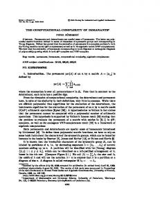
2.1. Local Search Operators for the VRP The most common local search methods designed for the VRP consider neighborhood structures defined by simple arc exchange moves [6]. In the general case, a k-exchange move involves the deletion of (up to) k arcs of the current solution and the generation of k new ones to produce the subsequent solution. The complexity of exhaustively examining the k-exchange neighborhood of a solution is O(nk), so that in practical local search methods the value of k rarely exceeds 3 or 4, because this would lead to excessive computational times [7]. Three common paradigms of simple and effective VRP local search operators, also used in the proposed methodology, are: (a) the 1-0 exchange (customer relocation), (b) the 1-1 exchange (customer exchange), and (c) the 2-opt move (route crossover) illustrated in Fig.1. The 1-0 exchange move (Fig. 1(a)) relocates a customer from its current position to another, by replacing three solution arcs. The 1-1 exchange (Fig. 1(b)) swaps the positions of a customer pair by removing four arcs and creating four new ones. Last, the 2-opt move involves the deletion and creation of an arc pair. The aforementioned local search operators can be characterized as 2exchange methods, although they involve the deletion and generation of more than two arcs (three for the 1-0 exchange, and four for the 1-1 exchange). This is because only two arcs have to be determined to fully describe a given move [7]. In specific, the 1-0 exchange of Fig.1 (a) can be fully described by the deleted arcs AB and DE, while arc BC is implicitly defined by the move mechanism. Analogously, the 1-1 exchange of Fig.1 (b) can be determined by the deleted arc pair AB and DE. The other two deleted arcs (EF and BC) are implicitly defined by the rationale of the

5

move. As a result, the cardinality of these neighborhoods is O(n2), and taking into account that their evaluation requires constant time [8], it can be easily seen that exhaustively examining one of these neighborhoods requires O(n2) computational effort. To accelerate local search algorithms, researchers have proposed several schemes for reducing the solution neighborhood cardinality and the mechanism of exploring the solution neighborhoods. In terms of the neighborhood cardinality, Glover and Laguna [9] introduce the candidate list strategies, which generate only a small subset of all tentative local search moves. Similarly, Coy et al. [10] propose a fixed length neighbor list for the Traveling Salesman Problem (TSP). Their method associates every vertex to a fixed number of neighboring vertices. Moves are evaluated, only if they lead to the creation of an arc connecting two neighboring vertices. Li et al. [5] extend this idea by considering a variable length neighbor list for solving the VRP. Toth and Vigo [7] propose another neighborhood reduction scheme based on the concept of granular neighborhoods. These neighborhoods do not contain moves leading to features not likely to belong to high quality solutions, and are dynamically adjusted by exploiting information collected during the search process. In the same context, Nagata and Bräysy [11] have proposed some local search limitation strategies for vehicle routing problems. The key idea is to restrict the neighborhood structures by considering only the tentative moves that lead to the creation of edges which are stored in a list. This list is dynamically updated through the search process using several policies proposed by the authors. Regarding the mechanism of neighborhood exploration, sequential search has been independently proposed by Lin and Kernighan [12], and Christofides and Eilon [13] for the TSP. The basic rationale of the sequential search concept is to prune the search as early as possible, so that a small subset of the tentative moves is evaluated. This pruning is achieved by calculating bounds to filter out the evaluation of cost-increasing tentative moves. More recent works aimed at accelerating local search methods for routing problems include the studies of Irnich et al. [14], and Irnich [15]. The former work provides sequential search implementations of several routing neighborhoods structures, and compares the efficiency of these implementations against classical lexicographic search approaches. The latter work proposes a unified modeling framework for routing problem variants with various complex side constraints. In methodological terms, the sequential search approach, presented in [14], is adapted to these complex-constrained routing problems. Pre-processing methods are also proposed to avoid increasing the computational complexity required for investigating feasibility. Apart from the simple arc exchange local search moves described above, researchers have also developed more complex neighborhood structures for the VRP. Ejection chain

6

approaches, originally proposed for the Traveling Salesman Problem by Glover [16], generate compound neighborhood structures, which encompass successions of interdependent moves, instead of simple moves or sequences of independent moves. Their application has proven to be effective also for the VRP model [17, 18]. Another compound move has been proposed by Osman [19]. It involves the combination of vertex insertions and exchanges between routes based on the 2-opt process. Gendreau et al. [20] propose a complex VRP move which consists of a simple vertex insertion, followed by a 3-opt or 4-opt exchange. As a last example of VRP complex neighborhoods, we mention the work of Xu and Kelly [21], which presents an original local search approach based on a network flow model that is used to simultaneously evaluate several customer ejection and insertion moves.

C

A

E

C

A

B

D

E

D

B

F

C

D

A

C

A

E

C

A

B

E

D

B

F

C

D

A B

B D (a) 1-0 exchange

(b) 1-1 exchange

Arcs Created

(c) 2-opt

Arcs Deleted

Figure 1 Simple Local Search Operators for the VRP

2.2. Local Search Metaheuristic Approaches for the VRP Several of the most effective VRP metaheuristic approaches make use of simple local search operators like those presented in 2.1. Rochat and Taillard [22] have proposed an adaptive memory framework for dealing with the VRP. Their approach makes use of a pool of routes which belong to a set of elite solutions. Routes are extracted from the pool to form new complete or partial solutions which are improved by means of a TS method that employs 1-1 and 1-0 vertex

7

exchanges. The obtained solutions are then used to update the route pool. Tarantilis and Kiranoudis [23], and Tarantilis [24] have also proposed a similar scheme for solving the CVRP. The key difference between their methods and the one of Rochat and Taillard [22] is that new partial solutions are built by combining promising vertex sequences (bones) present in the adaptive memory. These solutions are then improved by a TS procedure which makes use of the 1-0, 1-1 exchanges and 2-opt neighborhood structures. Li et al. [5] propose a record-to-record algorithm [25] for solving large scale routing problems. Their method investigates the neighborhoods of 1-0, 1-1 exchanges and 2-opt moves reduced by using the aforementioned variable-length neighbor list policy. Another effective local search based metaheuristic has been proposed by Toth and Vigo [7]. As mentioned above, they propose a TS method that explores drastically restricted neighborhoods. This is accomplished by ignoring moves that result into characteristics not likely to be part of a high-quality solution. The blend of local search operators used in their approach consists of four neighborhood structures: 1-1 exchange, 1-0 exchange, 2opt, and 2-point Or exchange which relocates two consecutive customers [26]. Reimann et al. [27] present an Ant System for solving the VRP. In specific, their approach decomposes the global VRP problem into TSP subproblems by clustering customer vertices into disjoint sets. Then, each subproblem TSP solution is optimized by the Savings Based Ant System which makes use of the 1-1 exchange and 2-opt moves. The total VRP solution is obtained by recombining the TSP solutions. Mester and Bräysy [28] present a metaheuristic development which combines the strengths of GLS and evolution strategies into an iterative framework. Their highly effective algorithm makes use of a composite local search method which consists of vertex exchanges, reinsertions and 2-opt moves, both for intra- and inter-route improvements. Finally, the work of Tarantilis et al. [29] is an example of how the 1-0, 1-1 exchange and 2-opt operators can be effectively modified for dealing with a routing variant which considers intermediate replenishment stops. These modified local search operators are integrated into a hybrid metaheuristic framework producing a highly effective algorithm.

3. The Proposed Local Search Methodology The proposed local search framework makes use of the static move descriptors which were briefly discussed in the introductory section. Here, we provide an analytic description of them, together with a thorough discussion on their behavior.

8

3.1. Local Search Static Move Descriptors As earlier mentioned, most local search operators designed for the VRP consider simple arc exchange moves for transiting from one solution to the other. To define such a move instance, one has to determine the move rule and the move point. The move rule corresponds to the move mechanism and is common for all move instances of the same neighborhood structure, while the move point expresses a constant set of problem features, where the move instance is applied to. Both the move rule and move point information is static, or in other words, independent of the current solution. A Static Move Descriptor (SMD) is an entity containing this information, and each instance of it can be interpreted as a particular move from one solution to another. An SMD instance does also contain the cost required to be applied. This cost is the only dynamic (or in other words, solution dependent) information, stored in an SMD instance. To more clearly introduce the SMD concept, we are going to present it for the particular local search operators used in our methodology, namely the 1-0 exchange, the 1-1 exchange, and the 2-opt move, illustrated in Fig.1.

1-0_SMD Instances n1 = 0 n2 = A

n1 = 00 n2 = A

n1 = B n2 = A

n1 = C n2 = A

n1 = D n2 = A

n1 = E n2 = A

n1 = 0 n2 = B

n1 = 00 n2 = B

n1 = A n2 = B

n1 = C n2 = B

n1 = D n2 = B

n1 = E n2 = B

n1 = 0 n2 = C

n1 = 00 n2 = C

n1 = A n2 = C

n1 = B n2 = C

n1 = D n2 = C

n1 = E n2 = C

n1 = 0 n2 = D

n1 = 00 n2 = D

n1 = A n2 = D

n1 = B n2 = D

n1 = C n2 = D

n1 = E n2 = D

n1 = 0 n2 = E

n1 = 00 n2 = E

n1 = A n2 = E

n1 = B n2 = E

n1 = C n2 = E

n1 = D n2 = E

Transformed Solution S1 0

D

A

0

00

C

B

E

Solution S 0

C

D

A

00

B

E

00

Transformed Solution S3

Transformed Solution S2

00

0

0

C

A

0

00

B

D

E

00

0

C

D

A

00

E

B

00

0

Figure 2 The mechanism of the move descriptors for the 1-0 exchange move

9

1-0 Exchange Static Move Descriptor The 1-0 exchange move (customer relocation), removes a customer vertex from its current position and reinserts it into a new one, as seen in Fig.1 (a). The move point of the SMD objects designed for the 1-0 exchange (denoted by 1-0_SMD) is a pair of two distinct vertices n1 and n2, while the move rule is: “Remove n2 from its current position and reinsert it after n1”. The 1-0_SMD applied in the case of Fig. 1(a) is the one corresponding to n1 = D and n2 = B. To exhaustively describe the 1-0 exchange neighborhood of a given solution, the creation of one 1-0_SMD instance for every possible move is required. It is easily seen that in total n · (n + K - 1) 1-0_SMD instances are necessary, where K is the number of vehicles present in the solution and represents the occurrences of the depot vertex in the solution vector. Figure 2 illustrates the move descriptor instances for a VRP of 5 customers and 2 vehicles. It also demonstrates the results of implementing three example 1-0_SMD instances to an arbitrary solution.

1-1_SMD Instances n1 = A n2 = B

n1 = A n2 = C

n1 = A n2 = D

n1 = A n2 = E

n1 = B n2 = C

n1 = B n2 = D

n1 = B n2 = E

n1 = C n2 = D

n1 = C n2 = E

Solution S 0

C

D

A

00

B

E

00

0

n1 = D n2 = E

Transformed Solution S1

Transformed Solution S2

0

A

D

C

00

B

E

00

0

0

C

E

A

00

B

D

00

0

Figure 3 The mechanism of the move descriptors for the 1-1 exchange move

10

1-1 Exchange Static Move Descriptor The 1-1 Exchange operator exchanges the positions of two customer vertices as seen in Fig 1(b). This operator has a symmetric nature because the solution effect of exchanging the positions of customers vi and vj is the same with that of exchanging the vj and vi positions. To exploit this symmetry, the move point of the descriptors generated for the 1-1 exchange (denoted by 1-1_SMD) consists of a pair of distinct customer vertices n1 and n2. The move rule is straightforward: “Exchange the positions of n1 and n2”. The 1-1_SMD instance corresponding to the move of Fig. 1(b) is the one corresponding to n1 = B and n2 = E. To exhaustively describe the 1-1 neighborhood of a given solution, one 1-1_SMD instance per customer pair must be generated. Thus, the total population of 1-1_SMD instances required is n! (2!( n − 2)!) . Figure 3 illustrates the 1-1 Exchange move descriptor instances for a VRP of 5 customers and 2 vehicles. It also demonstrates the results of implementing two example 1-1_SMD instances to an arbitrary solution.

2-opt_SMD Instances n1 = A n2 = B

n1 = A n2 = C

n1 = A n2 = D

n1 = A n2 = E

n1 = A n2 = 0

n1 = A n2 = 00

n1 = B n2 = C

n1 = B n2 = D

n1 = B n2 = E

n1 = B n2 = 0

n1 = B n2 = 00

n1 = C n2 = D

n1 = C n2 = E

n1 = C n2 = 0

n1 = C n2 = 00

n1 = D n2 = E

n1 = D n2 = 0

n1 = D n2 = 00

n1 = E n2 = 0

n1 = E n2 = 00

Solution S 00

B

E

00

0

C

D

A

0

n1 = 0 n2 = 00 Transformed Solution S1 00

B

D

A

0

C

E

00

Transformed Solution S3

Transformed Solution S2 0

00

D

A

0

0

C

B

E

00

00

B

E

00

0

A

D

C

0

Reversed Path

Figure 4 The mechanism of the move descriptors for the 2-opt move

11

2-opt Static Move Descriptor Both the inter- and intra-route 2-opt moves delete two arcs present in the solution, and replace them with two new ones. They exhibit symmetric behavior, because each combination of two deleted arcs defines a single 2-opt move (repetitions of arc pairs define identical moves). To statically express this symmetric behavior, the SMD proposed for the 2-opt move (denoted by 2-opt_SMD) has been designed as follows: The move point of a 2-opt_SMD object consists of two non-identical vertices n1 and n2, while the move rule suggests: “If n1 and n2 belong to different routes, connect vertices n1 and n2 to the paths beginning after vertex n2 and after vertex n1, respectively. Otherwise, if n1 and n2 belong to the same route and n2 precedes n1 in the route vector, swap the n1 and n2 values. Then, connect n1 to n2, by reversing the path lying between n1 and n2”. The 2-opt_SMD instance applied for the move of Fig.1(c) is the one corresponding to n1 = A and n2 = C (assuming that A and C belong to different routes). It can easily be seen that to exhaustively describe the 2-opt neighborhood of a given solution, in total

(n + K )! (2!(n + K − 2)!) 2-opt_SMD instances are necessary, where K is the number of routes present in the solution. Figure 4 illustrates the SMD mechanism of the 2-opt move for the 5customer, 2-route example VRP examined above.

3.2. The Cost of the Static Move Descriptors Apart from describing a particular move, every SMD instance does also contain the cost of implementing this move to a given solution. When a move is performed, only a limited part of the solution structure is modified. For the VRP local search operators described above, this modified part consists of a small subset of the solution arcs. Therefore, to keep the SMD cost labels valid, each time a local search operator is applied, one must evaluate the costs of the SMD instances that refer to the affected solution part. In other words, for the VRP model, rather than every SMD cost label, only those that involve the cost of the affected solution arcs have to be updated. To better present the mechanism of keeping the costs of the SMD instances updated, we provide Fig. 5 which illustrates how does the application of an inter-route 2-opt move affect the cost labels of the SMD instances for the 1-1 exchanges. The VRP problem presented in Fig. 5 involves 8 customers and 2 vehicles. The (inter-route) 2-opt_SMD applied in the case of Fig. 5 has n1 = B and n2 = D. It removes arcs DC and BG, which are replaced by DG and BC. This particular move does not affect the cost of every 1-1_SMD instance. Instead, it modifies only those whose cost depends on the arcs deleted - and generated - by the 2-opt move (these arcs are written in bold characters in Fig. 5). In total, the costs of 22 1-1_SMD instances have to be reevaluated (indicated by the shadowed areas in Fig. 5). The remaining 6 instances remain unaffected and therefore their re-calculation is unnecessary. A more thorough look on the subset

12

of affected cost labels can provide the formal rule of cost update for the 1-1_SMD instances, when an inter-route 2-opt_SMD is applied to a given solution: “When an inter-route 2-opt_SMD instance with n1 = 2-opt_n1 and n2 = 2-opt_n2 is applied to a given solution S, the costs of the 11_SMD instances with their n1 or n2 equal to 2-opt_n1, 2-opt_n2, succ(2-opt_n1) or succ(2-opt_n2), are modified and have to be updated, where succ(v) denotes the successor of v in solution S. In the example case of Fig. 5, we have 2-opt_n1 = B and 2-opt_n2 = D, with succ(B) = G and succ(D) = C. Therefore, the 1-1_SMD instances that must be re-evaluated have their n1 or n2 value equal to B, D, G or C, as seen in Fig. 5. To apply the proposed methodology, one needs to deduce all formal rules of cost update for the local search operators applied. These rules can be interpreted as the way in which the neighborhood structures both affect themselves, and interact with each other. The rules for updating the SMD instances of the three local search operators used in our methodology are summarized in Table 1. Each row consists of the SMD instances that must be updated when a particular local search operator is applied. The first row, for instance, suggests that when a 10_SMD instance with n1 = A and n2 = B is applied to a particular solution S, the following SMD instances must be updated: a) 1-0_SMD instances with n1 equal to A, pred(B), or B b) 1-0_SMD instances with n2 equal to A, succ(A), pred(B), B, succ(B) c) 1-1_SMD instances with n1 or n2 equal to A, succ(A), pred(B), B, or succ(B) d) 2-opt_SMD instances with n1 or n2 equal to A, pred(B), or B, where pred(v) and succ(v) denote the predecessor and successor of vertex v in solution S, respectively. From the update rules presented in Table 1, we see that when a 1-0 and 1-1 exchange move is performed, the total number of SMD cost labels that must be updated is linearly correlated to the instance size n, or to be more precise with n′ = n + K, where K represents the routes present in the current solution. When a 2-opt move is performed, the population of SMD instances to be updated depends on the state of the solution where the particular 2-opt move is applied to. However, loosely speaking, the affected SMD instances are confined to those that either their n1 or n2 vertex belongs to the routes (or route) involved in the 2-opt move applied. The value of this is obvious: within an iterative local search framework, encoding the tentative moves into SMD instances drastically reduces the - per iteration - calculations required to exhaustively evaluate the cost of solution neighborhoods. In the particular case of the 1-0 and 1-1 exchange quadratic O(n2) operators, applied in the proposed framework, the use of the SMD concept allows neighborhoods to be exhaustively evaluated at the expense of O(n) complexity.

13

Table 1 Rules for updating the SMD cost tags when a local search operator is applied SMD Instances to be Updated SMD Instance Applied

1-0 Exchange

1-0 Exchange n1 = A n2 = B

n1=A. n1=pred(B). n1=B.

1-1 Exchange n1 = A n2 = B

n1=pred(A). n1=A. n1=pred(B). n1=B.

1-1 Exchange

n2=A. n2=succ(A). n2=pred(B). n2=B. n2=succ(B). n2=pred(A). n2=A. n2=succ(A). n2=pred(B). n2=B. n2=succ(B).

n1=A OR n2=A. n1=succ(A) OR n2=succ(A). n1=pred(B) OR n2=pred(B). n1=B OR n2=B. n1=succ(B) OR n2=succ(B). n1=pred(A) OR n2=pred(A). n1=A OR n2=A. n1=succ(A) OR n2=succ(A). n1=pred(B) OR n2=pred(B). n1=B OR n2=B. n1=succ(B) OR n2=succ(B).

2-opt

n1=A OR n2=A. n1=pred(B) OR n2=pred(B). n1=B OR n2=B. n1=pred(A) OR n2=pred(A). n1=A OR n2=A. n1=pred(B) OR n2=pred(B). n1=B OR n2=B.

Interroute 2-opt n1 = A n2 = B

n1=A. n1=B.

n2=A. n2=succ(A). n2=B. n2=succ(B).

n2=A OR n2=A. n2=succ(A) OR n2=succ(A). n2=B OR n2=B. n2=succ(B) OR n2=succ(B).

n1=A OR n2=A. n1=B OR n2=B. ( n1 ∈ fst(A), n2 ∈ sec(A) OR n2 ∈ fst(A), n1 ∈ sec(A) ). ( n1 ∈ fst(A), n2 ∈ sec(B) OR n2 ∈ fst(A), n1 ∈ sec(B) ). ( n1 ∈ fst(B), n2 ∈ sec(A) OR n2 ∈ fst(B), n1 ∈ sec(A) ). ( n1 ∈ fst(B), n2 ∈ sec(B) OR n2 ∈ fst(B), n1 ∈ sec(B) ).

IntraRoute 2-opt n1 = A n2 = B

n1 ∈ rev(A,B). n1=A.

n2=A. n2=succ(A). n2=B. n2=succ(B).

n2=A OR n2=A. n2=succ(A) OR n2=succ(A). n2=B OR n2=B. n2=succ(B) OR n2=succ(B).

n1=A OR n2=A. n1 ∈ rev(A,B) OR n2 ∈ rev(A,B).

pred(v): the predecessor of vertex v before the move application, succ(v): the successor of vertex v before the move application. fst(v): the route segment originating from the depot and terminating at the predecessor of vertex v, before the move application, sec(v): the route segment originating from the successor of vertex v and terminating at the depot, before the move application. For the application of Intra-Route 2-opt SMD, assume that A precedes B in the route vector, before the move is implemented rev(A,B): the reversed route path between vertices A and B (beginning from the successor of A and ending at B, see Fig. 4) The ‘,’ character can be interpreted as the logic operator AND, The ‘.’ character separates each cost update rule.

14

1-1 Exchange SMD (Before applying 2-opt Move)

n1=A

n2=B

n2=C

n2=D

n2=E

n2=F

n2=G

n2=H

c(A,B) = 0B+BD+ EA+AG(0A+AD+ EB+BG)

c(A,C) = 0C+CD+ DA+AH(0A+AD+ DC+CH) c(B,C) = EC+CG+ DB+BH(EB+BG+ DC+CH)

c(A,D) = 0D+DA+ AC(0A+AD+ DC) c(B,D) = ED+DG+ AB+BC(EB+BG+ AD+DC) c(C,D) = AC+CD+ DH(AD+DC+ CH)

c(A,E) = 0E+ED+ 00A+AB(0A+AD+ 00E+EB) c(B,E) = 00B+BE+ EG(00E+EB+ BG) c(C,E) = DE+EH+ 00C+CB(DC+CH+ 00E+EB) c(D,E) = AE+EC+ 00D+DB(AD+DC+ 00E+EB)

c(A,F) = 0F+FD+ GA+A00(0A+AD+ GF+F00) c(B,F) = EF+FG+ GB+B00(EB+BG+ GF+F00) c(C,F) = DF+FH+ GC+C00(DC+CH+ GF+F00) c(D,F) = AF+FC+ GD+D00(AD+DC+ GF+F00)

c(A,G) = 0G+GD+ BA+AF(0A+AD+ BG+GF) c(B,G) = EG+GB+ BF(EB+BG+ GF) c(C,G) = DG+GH+ BC+CH(DC+CH+ BG+GF) c(D,G) = AG+GC+ BD+DF(AD+DC+ BG+GF)

c(A,H) = 0H+HD+ CA+A0(0A+AD+ CH+H0) c(B,H) = EH+HG+ CB+B0(EB+BG+ CH+H0) c(C,H) = DH+HC+ C0(DC+CH+ H0) c(D,H) = AH+HC+ CD+D0(AD+DC+ CH+H0)

c(E,F) = 00F+FB+ GE+E00(00E+EB+ GF+F00)

c(E,G) = 00G+GB+ BE+EF(00E+EB+ BG+GF)

c(E,H) = 00H+HB+ CE+E0(00E+EB+ CH+H0)

c(F,G) = BF+FG+ G00(BG+GF+ F00)

c(F,H) = GH+H00+ CF+F0(GF+F00+ CH+H0)

n1=B

n1=C

n1=D

n1=E

n1=F

Affected Part of the Solution

0

A

D

C

H

0

00

E

B

G

F

00

c(G,H) = BH+HF+ CG+G0(BG+GF+ CH+H0)

n1=G

2-opt_SMD n1 = B, n2 = D

Delete Arcs: DC BG

c(B,D)= DG + BC(DC - BG)

Create Arcs: DG BC

Apply

1-1 Exchange SMD (After applying 2-opt Move)

n1=A

n1=B

n1=C

n1=D

n1=E

n1=F

n1=G

n2=B

n2=C

n2=D

n2=E

n2=F

n2=G

n2=H

c(A,B) = 0B+BD+ EA+AC(0A+AD+ EB+BC)

c(A,C) = 0C+CD+ BA+AH(0A+AD+ BC+CH) c(B,C) = EC+CB+ BH(EB+BC+ CH)

c(A,D) = 0D+DA+ AG(0A+AD+ DG) c(B,D) = ED+DC+ AB+BG(EB+BC+ AD+DG) c(C,D) = BD+DH+ AC+CG(BC+CH+ AD+DG)

c(A,E) = 0E+ED+ 00A+AB(0A+AD+ 00E+EB) c(B,E) = 00B+BE+ EC(00E+EB+ BC) c(C,E) = BE+EH+ 00C+CB(BC+CH+ 00E+EB) c(D,E) = AE+EG+ 00D+DB(AD+DG+ 00E+EB)

c(A,F) = 0F+FD+ GA+A00(0A+AD+ GF+F00) c(B,F) = EF+FC+ GB+B00(EB+BC+ GF+F00) c(C,F) = BF+FH+ GC+C00(BC+CH+ GF+F00) c(D,F) = AF+FG+ GD+D00(AD+DG+ GF+F00)

c(A,G) = 0G+GD+ DA+AF(0A+AD+ DG+GF) c(B,G) = EG+GC+ DB+BF(EB+BC+ DG+GF) c(C,G) = BG+GH+ DC+CF(BC+CH+ DG+GF) c(D,G) = AG+GD+ DF(AD+DG+ GF)

c(A,H) = 0H+HD+ CA+A0(0A+AD+ CH+H0) c(B,H) = EH+HC+ CB+B0(EB+BC+ CH+H0) c(C,H) = BH+HC+ C0(BC+CH+ H0) c(D,H) = AH+HG+ CD+D0(AD+DG+ CH+H0)

c(E,F) = 00F+FB+ GE+E00(00E+EB+ GF+F00)

c(E,G) = 00G+GB+ DE+EF(00E+EB+ DG+GF)

c(E,H) = 00H+HB+ CE+E0(00E+EB+ CH+H0)

c(F,G) = DF+FG+ G00(DG+GF+ F00)

c(F,H) = GH+H00+ CF+F0(GF+F00+ CH+H0)

Affected Part of the Solution

0

A

D

G

F

00

00

E

B

C

H

0

c(G,H) = DH+HF+ CG+G0(DG+GF+ CH+H0)

Figure 5 The effect of a 2-opt move on the 1-1 exchange SMD instances

15

3.3. Keeping the SMD Instances Sorted To perform local search using the best admissible move strategy, apart from evaluating the costs required for implementing every tentative move, one must identify the particular move minimizing the cost involved. Accordingly, when using the SMD instances for encoding tentative moves, the particular SMD instance with the minimum cost label must be identified and applied. A straightforward way to do so would be to go through every SMD instance in order to locate the minimum cost one. However, this would require O(n2) complexity because the total population of SMD instances is O(n2), as earlier presented. To avoid this complexity increase, we use a priority queue data structure, called Fibonacci Heap introduced by Fredman and Tarjan [30]. This structure is used for keeping the SMD instances sorted according to their cost labels and provides the following key capabilities: a) it returns the lowest cost SMD at constant time, b) allows SMD instance deletions in O(log m), where m = n2 (corresponding to the total number of SMD instances), and c) allows SMD instance insertions at constant time. The role of the first capability is obvious, as it is directly related to the selection of the best tentative move. The second and third characteristics of the Fibonacci Heap are important for the process of updating the cost labels of the affected SMD instances, when a local search operator is applied. In particular, the process of updating the cost of a single SMD instance involves three steps: delete the SMD instance from the data structure, modify its cost label, and finally insert it back into the data structure. Since the cost modification (for the considered VRP local search operators), and insertion steps are executed in O(1), the overall complexity of a single update process is bounded by the deletion step which requires logarithmic complexity (O(log n2) = O(2 log n)). The application of a 1-0 and 1-1 exchange operator updates the cost of O(n) SMD instances. Thus, for these particular move types, the required computational complexity -per iteration- for keeping all SMD instances updated and sorted is O(n log n). For the 2-opt move, the space complexity of the modified SMD instances cannot be explicitly defined. However, assuming that l denotes the affected SMD instances (where in the general case l < n2, and l 0) go to 17 14 apply the move represented by toBeApplied to Solution S 15 update the cost labels of the SMD instances affected by toBeApplied 16 end do 17 return S

Figure 6 The Local Search method

17

3.5. Feasibility Issues To empirically determine the number of SMD instances that need to be extracted from their Fibonacci Heap until the first feasible one is obtained, and compare this number against the problem scale, we performed the following experiment: for 32 problems in total (described in detail in subsection 5.1), we executed a local search method like the one presented in Fig. 6, using all three presented local search operators. In specific, each iteration of lines 7-16 involved a randomly selected neighborhood structure, with each structure having the same probability of being selected. To cover a wider region of the solution space, so that more representative results are obtained, we also applied a tabu strategy which forbids the application of SMD instances corresponding to performed move reversals. The tabu horizon considered was 10 iterations per move type. The termination condition was set to the completion of 50,000 iterations. For each neighborhood structure, we measured the -per iteration- average number of SMD instances that had to be extracted from the corresponding Fibonacci Heap, before the first admissible SMD instance was obtained, or in other words the required iterations of the loop of lines 9-11 in Fig. 6. Note that for the presented experimental procedure, an admissible SMD instance apart from the feasibility requirement must also be non-tabu.

1-0 Exchange

1-1 Exchange

CVRP

DCVRP

SMD instances extracted until the first admissible SMD was obtained

600

2-opt 2000

50 40

400

1500

30 1000 20

200

500

10 0

0 200

300

400

500

0 200

300

400

500

14

20

300

400

500

1000

12

16

200

800

10 12

8

600

8

6

400

4 4

200

2

0

0 150

450

750

1050

0 150

450

750

1050

150

450

750

1050

n: Problem Size

Figure 7 Number of SMD instances extracted until the first admissible is obtained against problem size

18

From the experimental results illustrated in Fig. 7, we can see that the extracted SMD instances for the 1-0 and 1-1 move types are significantly fewer than the 2-opt ones. This is because the inter-route 2-opt operator swaps route segments that contain large customer sets causing a significant effect in terms of the solution feasibility status. The number of extracted 1-0 and 2-opt SMD instances illustrates a slight positive correlation with the instance size, however the growth rate does not exhibit any quadratic behavior. For the 1-1 exchange, the number of extracted SMD instances depended on the instance characteristics exclusively, without demonstrating any correlation to the instance size. Finally, for all three local search operators and for both problem versions (CVRP and DCVRP) the number of extracted SMD instances is insignificant compared to the total SMD instance populations. In specific, let rextr denote the ratio between the average extracted SMD instances, and the total number of SMD instances of a given move type. For the CVRP model, the rextr ratio ranged within [0.131%, 0.386%], [0.020%, 0.100%], and [0.897%, 2.253%], for the 1-0 exchange, 1-1 exchange and 2-opt moves, respectively. For the DCVRP model, the aforementioned rextr ratios ranged within [0.000%, 0.006%], [0.001%, 0.037%], and [0.035%, 0.359%], respectively. The ranges of the rextr value indicate that the procedure of extracting SMD instances from their Fibonacci Heaps, to obtain the first admissible one, does not significantly contribute to the computational effort required by the overall local search framework. At this point, we should note that as the SMD instances (tentative moves) are sorted according to their cost labels, the proposed scheme checks the feasibility of only the high quality moves which are the actual candidates for being applied. This characteristic can drastically reduce the computational time dedicated for feasibility evaluations of problem models with complex constraints, because unproductive feasibility checks are avoided. Regarding the feasibility issues, if tunneling through infeasible solution space is allowed, or constraints are very tight so that feasibility evaluation determines the total computational effort, the SMD design could also incorporate feasibility information. This could be achieved, for instance, with the use of excess penalties (for infeasible tunneling), or even dummy penalty cost labels for the infeasible SMD instances. In this case however, the SMD cost update rules for the application of a move must be appropriately designed to reflect the changes that this specific move has caused in terms of the dynamic feasibility status of the SMD instances.

3.6. The Acceleration Role of the Static Move Descriptors To present the acceleration role of the proposed SMD representation, the following experiment was performed: we executed the local search method described in 3.4 using the new SMD

19

representation of tentative moves, and with the classic move representation. The local search operator employed was the quadratic 1-0 exchange. The termination condition used was the completion of 50,000 iterations. To avoid being trapped in local optima, deteriorating moves were allowed, and move reversals were eliminated using the tabu strategy. In terms of the cost of the final solutions, both methods produced identical results, as the exact same search rules were applied. The two compared methods did only differ on the representation used for evaluating solution neighborhoods, and therefore on the total CPU effort required.

CPU Time for 50000 iterations (sec)

2500

2000 Classic Representation

1500

1000

SMD reprentation

500

0 200

400

600 800 n: Problem Size

1000

1200

Figure 8 The acceleration role of the SMD representation

350

CPU time for 50000 iterations (sec)

300 250 200 150 100 50 0 0

500

1000

1500

2000

2500

3000

3500

4000

n log(n) n: Problem Size

Figure 9 The linearithmic behavior of the search process using the SMD concept

20

The comparative results obtained by the aforementioned experimental procedure are summarized in Fig. 8. As seen from Fig. 8, the computational times required by both representations are comparable for problem scales of up to 350-400 customers. This is because the acceleration effect of the SMD concept is counterbalanced by the extra computations performed internally to the Fibonacci Heap structure. However, as the problem scale becomes larger, the CPU time required by the classic representation exhibits quadratic growth. On the contrary, the CPU time required by the search process with the use of the SMD representation presents a linearithmic growth rate, as more clearly illustrated in Fig. 9. Note that for the problem instance of 1,200 customers, the complexity reduction achieved by the use of the SMD representation reduces the total time of the search process by a remarkable 87.96% (classic representation: 2,485.89 sec, SMD representation: 299.36 sec).

4. A VRP Tabu Search Based on the SMD Concept In this Section, we propose a VRP metaheuristic which exploits the SMD representation of solution neighborhoods analytically described in Section 3. Let PSMDA (Penalized Static Move Descriptors Algorithm) denote the proposed solution approach. The central rationale of PSMDA is to penalize the cost labels of the SMD instances to diversify the search process. In terms of the speed of the algorithm, except for the acceleration role of the SMD strategy, we also apply a neighborhood reduction policy similar to the granularity concept introduced by Toth and Vigo (2003). Note that as the PSMDA makes use of the SMD local search engine, the CPU time demanded -per iteration- by the proposed algorithm exhibits almost linearithmic growth with the instance size. The PSMDA metaheuristic is presented in detail in the following subsections.

4.1. Initializing the PSMDA Metaheuristic Methodology To obtain an initial VRP solution, we apply the weighted savings heuristic originally proposed by Paessens (1988). The savings function used is: s(vi, vj) = ci0 + c0j – g · cij + f · | ci0 - c0j |,

(1)

where the f and g parameter values are uniformly distributed within [0, 1] and (0, 3], respectively, as proposed by Paessens [31]. The PSMDA framework makes use of the 1-0, 1-1 exchange and 2-opt local search operators (denoted by NS1, NS2 and NS3, respectively) described in Section 3, thus it is initiated by generating the SMD instances for these three neighbourhood structures. To reduce the total amount of generated SMD instances, and therefore the calculations needed for keeping their cost labels updated, we followed a strategy similar to the granularity concept of Toth and Vigo [7].

21

The main idea of this neighbourhood reduction scheme is to create SMD instances for encoding only those moves that are likely to produce high-quality solutions. To do so, we calculate a threshold cost θ as:

θ =β⋅

z(S 0 ) , n + K0

(2)

where z(S0), and K0 denote the cost and the number of routes of the initial solution S0, respectively, and β is the sparsification parameter set to 2.5, as proposed by Toth and Vigo [7]. Then, for all three local search operators, an SMD instance with n1 = i and n2 = j is generated, if at least one of the following holds: cij ≤ θ, i = 0, j = 0. The application of the aforementioned move filtering criterion excludes poor quality moves from the search process and drastically accelerates the overall algorithm. By the term poor quality moves, we mean those moves that are highly unlikely to produce a good-quality solution, for instance, swapping the positions of a distant customer pair (1-1 exchange), or generating an arc connecting two remote customers (1-0 exchange). With each SMD instance smd, are associated two cost labels, namely smdCost, and smdPenCost. As their name suggests, smdCost represents the actual cost of the tentative move encoded in smd, while smdPenCost corresponds to this actual cost augmented via a penalization policy which is explained in the following. Then, for each neighbourhood structure NSi (i = 1, 2, 3) two Fibonacci Heaps FHi and PenFHi are created. The former heap (FHi) is responsible for keeping the SMD instances of NSi sorted according to their smdCost label, while the latter (PenFHi) keeps these instances sorted according to their penalized cost label smdPenCost. Every SMD cost label is evaluated (in terms of the initial solution S0), and every SMD instance is inserted into the appropriate Fibonacci Heap. Note that in the beginning smdPenCost = smdCost, for every instance smd. After the SMD encoding has been prepared, the core of the PSMDA approach is ready to be executed.

4.2. The Central Rationale of the PSMDA Metaheuristic The central idea of PSMDA is to perform diverse local search moves, so that the search is driven to various regions of the solution space. To do so, we exploit the design of SMD instances for mapping local search moves. As mentioned in Section 3, every SMD instance contains a move point. This point represents a set of problem features where the encoded move is applied to. In the case of the examined neighbourhood structures, the move point consists of a vertex pair n1 and n2. When an SMD instance with n1 = A and n2 = B is applied, the method performs structural modifications at the proximity of vertices A and B. To quantify this information, for every vertex

22

ni, we introduce a counter counti. This counter is responsible for keeping track of the number of times that an SMD instance with either its n1 or n2 value equal to ni has been implemented, and can be interpreted as the frequency with which the search has been conducted into the proximity of ni. The penalized cost label smdPenCost of an SMD instance with n1 = A and n2 = B is augmented by a penalty term proportionate to the (countA + countB) frequency metric. In this way, if one selects the SMD instances to be applied according to their penalized cost labels, the interest of the overall search is spread across every vertex of the problem, and is not confined into the proximity of small vertex subsets.

4.3. The Core of the PSMDA Solution Approach The PSMDA approach is a local search metaheuristic which begins the conducted search from the solution produced by the Paessens construction heuristic described in 4.1. At each iteration, the method performs the move represented by the SMD instance selected to be applied and denoted by app_smd. To determine the app_smd instance, the following procedure is used: From all three FHi (i = 1, 2, 3) (containing the SMD instances sorted according to their non-penalized cost labels), the lowest cost SMD instance np_smd is identified. If np_smd represents a move which improves the best solution found so far, the method applies this move (app_smd = np_smd). Otherwise, one of the examined neighbourhood structures (NS1, NS2, and NS3) is randomly selected. As seen in Table 1, the computations necessary for updating the costs of the SMD instances are linearly correlated to the instance size, when the 1-0 and 1-1 exchange moves are applied, whereas the implementation of a 2-opt move requires a greater number of SMD cost label updates. Therefore, to achieve an overall fast algorithmic behavior (keep the complexity as close to O(n log n) as possible), without significant loss of effectiveness, we limited the probability of 2-opt selection to 10%. The 1-0 and 1-1 exchange neighbourhood structures equally share the rest 90% probability of being selected. Let NSi denote the selected structure. Then, a uniformly distributed random variable fromPen is generated within the range [0, 1]. If fromPen < freqPen, the best SMD instance stored in PenFHi (containing the SMD instances of NSi sorted according to their penalized cost labels) and denoted by p_smd is selected to be applied (app_smd = p_smd). Otherwise, if fromPen ≥ freqPen, the move encoded by np_smd is performed (app_smd = np_smd). Note that apart from the diversification role of the penalization policy, we also use a tabu list which forbids move reversals, for a horizon of tabuTen iterations. Furthermore, our approach does not allow tunneling through infeasible regions. Therefore, the best SMD instances p_smd and np_smd extracted from the corresponding

23

Fibonacci Heaps, must both be non-tabu (unless the encoded move improves the best solution found), and satisfy the feasibility constraints.

Solution PSMDA (Solution S) Neighborhood Structure NSi double z, z* Solution S* SMD app_smd, np_smd, p_smd Fibonacci Heap FHi, PenFHi --Initialization generate the SMD instances for the neighborhood structures examined calculate the cost tags of the SMD instances for S insert the generated instances into the appropriate Fibonacci Heap --Improvement Phase while (termination condition = false) --Move Selection np_smd = best feasible non-tabu SMD instance extracted from all three FHi (i = 1, 2, 3) if (z + np_smdCost < z*) app_smd = np_smd else Select NSi from (NS1, NS2, NS3) randomly generate fromPen in [0, 1] if (fromPen < freqPen) p_smd = best feasible non-tabu SMD instance extracted from PenFHi app_smd = p_smd else app_smd = np_smd end if end if --Move Application apply app_smd to S z = z + app_smdCost declare the SMD reversals of app_smd tabu for tabuTen iterations let app_n1 and app_n2 denote the n1 and n2 vertices of app_smd countapp_n1 = count app_n1 + 1, countapp_n2 = count app_n2 + 1 for every affected SMD smd (following the update rules of Table 1) remove smd from its Fibonacci Heaps smdCost = calculate the cost of smd according to the new solution S let smd_n1 and smd_n2 denote n1 and n2 vertices of smd smdPenCost = smdCost + (countsmd_n1 + countsmd_n2) pen reinsert smd to the Fibonacci Heaps end for if (z < z*) S* = S z* = z end if end while return S*

Figure 10 Pseudocode of the PSMDA metaheuristic

24

After the SMD instance app_smd is identified, the search implements the corresponding move to obtain the subsequent solution. Let A and B denote the vertex pair of app_smd. The counters countA and countB are both augmented by 1, and the method applies the SMD cost update rules summarized in Table 1, for keeping every SMD cost tag updated according to the status of the new solution. The penalized cost tag of an SMD instance smd with n1 = A and n2 = B is evaluated as: smdPenCost = smdCost + (countA + countB) · pen,

(3)

where pen is a penalization parameter. From the update rules of Table 1, note that independently of the local search operator applied, every SMD instance with either its n1 or n2 value equal to A and B, is updated. Thus, all penalized cost tags are appropriately modified using the augmented countA and countB frequency values. The PSMDA method is executed until a certain termination condition is reached by returning the best solution obtained through the progress of the search. Fig. 10 provides the pseudocode of the PSMDA solution approach, using the same notation as in the verbal description of the method.

5. Computational Results of the PSMDA Metaheuristic To assess the performance and determine the parameter setting of the PSMDA strategy, we tested it on 32 large and very large scale VRP benchmark instances. Here, we provide some details on these benchmark instances, followed by a discussion on the PSMDA standard parameter setting. Finally, we provide the solution values obtained by the PSMDA together with the computational times involved. Apart from the 32 VRP benchmark instances, we also solved four real-world test problems each involving 3,000 customers. All instances and best solutions obtained are available at http://users.ntua.gr/ezach/.

5.1 Benchmark Instances Since the central aim of the present article is to propose a strategy for reducing the complexity of neighbourhood evaluations, PSMDA was tested on large scale VRP benchmark instances. In specific, we used the set of 20 large scale instances (200-483 customers) proposed by Golden et al. [25], and the set of 12 very large scale instances (560-1200 customers) introduced by Li et al. [5]. Note that we maintain the same problem ordering (problem 1 to 32), as given in the aforementioned works. The cost matrices for all 32 examined test problems are obtained by calculating the Euclidean distances between vertex locations. Problems 9-20 are pure CVRP instances, while problems 1-8 and 21-32 impose route length restrictions. Table 2 summarizes the details of all 32 test problems.

25

Table 2 Benchmark instances used for testing the proposed strategy Pr. 1 2 3 4 5 6 7 8 9 10 11 12 13 14 15 16 17 18 19 20

n 240 320 400 480 200 280 360 440 255 323 399 483 252 320 396 480 240 300 360 420

Large CVRP td Q 4,800 550 6,400 700 8,000 900 9,600 1000 4,000 900 5,600 900 7,200 900 8,800 900 13,429 1,000 15,195 1,000 16,980 1,000 18,701 1,000 25,136 1,000 28,672 1,000 32,244 1,000 35,772 1,000 4,320 200 5,400 200 6,480 200 7,560 200

D 650 900 1,200 1,600 1,800 1,500 1,300 1,200 -

Pr. 21 22 23 24 25 26 27 28 29 30 31 32

Very Large CVRP n td Q 560 11,200 1,200 600 12,000 900 640 12,800 1,400 720 14,400 1,500 760 15,200 900 800 16,000 1,700 840 16,800 900 880 17,600 1,800 960 19,200 2,000 1,040 20,800 2,100 1,120 22,400 2,300 1,200 24,000 2,500

D 1,800 1,000 2,200 2,400 900 2,500 900 2,800 3,000 3,200 3,500 3,600

n: number of customers, td: total demand of customers, Q: vehicle capacity, D: maximum route cost

5.2 Parameter Setting The PSMDA framework contains three parameters, namely freqPen, pen and tabuTen, the setting of which has to be determined before it is executed. The freqPen and pen parameters play a central role on the behavior of the algorithm, because they control the interplay between the intensification and diversification of the conducted search. In specific, freqPen defines the frequency with which moves are selected according to their penalized SMD cost, and pen controls the penalization terms (3) used to augment the cost of the SMD instances. Obviously, these two parameters jointly affect the search behavior. To avoid complex tuning experiments, we conducted preliminary algorithmic executions on all benchmark instances, using various rational pen values, and we observed that the best algorithmic performance was observed for freqPen values within the range [0.7, 0.9]. Therefore, the freqPen was fixed at 0.8, which injected satisfactory diversification into the search, and also let the algorithm intensify into promising solution regions. Having set freqPen to 0.8, we then experimented with the pen parameter. The setting of pen depends on both the cost matrix and the solution characteristics of the instance examined. To capture this correlation, pen was expressed according to the following relation: pen = μ · θ, where θ is the granular threshold introduced in (2). Then, we solved all benchmark instances with values of μ taken from [0.001, 0.01]. The best algorithmic behavior was

26

consistently observed for μ values between 0.004 and 0.008. Following this, pen was set to 0.006·θ. Regarding the number of iterations for which move reversals are declared tabu, we used tabuTen = 30, as suggested in the work of Tarantilis [24], for instances involving up to 500 customers. For the very large scale problems, with the customer population varying from 560 to 1,200, we used tabuTen = 60, which proved to be adequately high to eliminate cycling phenomena.

5.3 Results on CVRP Benchmark Instances To assess the performance of PSMDA, we solved all 32 benchmark instances 10 times with the standard parameter setting specified in 5.2. Each of the 10 algorithmic executions involved different initial solutions, because of the stochastic setting of f and g parameters (1). The termination condition used was reaching 30 CPU minutes for instances of up to 299 customers, 45 minutes for instances of up to 500 customers, and 90 minutes for the very large scale instances involving from 560 to 1,200 customers. Table 3 summarizes the results obtained, while Table 4 compares the best solution scores obtained by PSMDA to those achieved by some of the most effective published VRP metaheuristic approaches, and the best known solution for the examined instances. As seen in Table 3, the PSMDA has shown adequate stability, as for all 32 benchmark instances the average solution scores achieved over the 10 runs were very close the best ones. In specific, the average percent deviation between the best solution cost and the average one was limited to a satisfactory 0.19%. In terms of the CPU effort, PSMDA proved to be consistent, as the run time for obtaining the highest quality solution scores were close to the average run time for reaching the best solution, for all 10 algorithmic executions. Note also that the CPU time required by PSMDA does not exhibit quadratic growth with the instance size. Table 4 compares the best solution scores obtained by PSMDA with those reached by some of the most effective VRP algorithms ever proposed. It also presents a comparison between PSMDA solutions and the best known solutions (BKS column) for each benchmark instance. Note that some BKS values have not been obtained by any algorithmic approach. Instead, they have been visually estimated by exploiting their symmetric structure. PSMDA managed to improve 6 out of the 32 best-known solutions, and matched the best-known solutions for 5 test problems. The average percent gap of the PSMDA method and the previously best-known solutions is limited to a satisfactory 0.041% (0.061% for the large scale, and 0.008% for the very large scale instances). The greatest solution improvement was observed for the 760-customer

27

instance 25 (-0.474%), whereas the worst performance was recorded for the 1200-customer problem 32 (0.714%). In terms of PSMDA relative performance against the four presented highly effective solution approaches, we see that the average percent deviation between the PSMDA and the best algorithmic scores is restricted to 0.028% (0.042% for the large scale, and 0.004% for the very large scale instances). It also proved to be fairly robust, as the worst gap between a PSMDA and a previously reported algorithmic solution value was 0.688% (Instance 32).

Table 3 PSMDA results on the benchmark instances LS 1 (240) 2 (320) 3 (400) 4 (480) 5 (200) 6 (280) 7 (360) 8 (440) 9 (255) 10 (323) 11 (399) 12 (483) 13 (252) 14 (320) 15 (396) 16 (480) 17 (240) 18 (300) 19 (360) 20 (420)

K

%gap

5,637.99 8,457.92 11,036.22 13,632.59 6,460.98 8,412.90 10,192.47 11,674.43 584.66 739.86 919.52 1,110.65 860.44 1,083.55 1,344.41 1,623.42 708.94 997.74 1,370.77 1,829.57

Cavg

5,626.81 8,447.92 11,036.22 13,624.53 6,460.98 8,412.90 10,169.26 11,651.67 581.28 738.57 916.99 1,105.93 858.45 1,081.05 1,341.46 1,617.48 707.76 996.55 1,366.75 1,824.46

Cbest

9 10 10 10 5 7 9 10 14 16 18 19 26 30 33 37 22 27 33 38

0.20 0.12 0.00 0.06 0.00 0.00 0.23 0.20 0.58 0.18 0.28 0.43 0.23 0.23 0.22 0.37 0.17 0.12 0.29 0.28 0.21

16,230.83 14,607.81 18,824.94 21,422.36 16,840.05 24,012.13 17,495.68 26,614.71 29,195.72 31,808.08 34,375.96 37,248.39

16,212.83 14,587.12 18,801.13 21,389.43 16,822.09 23,977.73 17,471.33 26,566.04 29,154.34 31,742.64 34,330.94 37,182.88

10 15 10 10 19 10 20 10 10 10 10 11

avg VLS 21 (560) 22 (600) 23 (640) 24 (720) 25 (760) 26 (800) 27 (840) 28 (880) 29 (960) 30 (1040) 31 (1120) 32 (1200)

CPUavg

907.7 1,249.4 1,164.0 1,019.0 989.6 1,091.6 1,885.5 1,657.4 854.0 1,635.3 1,418.8 1,197.5 1,214.6 1,198.2 1,676.2 1,327.0 1,119.8 1,364.3 2,278.8 1,424.9 1,333.7

CPUbest

938.7 1,858.2 1,184.7 1,798.2 810.4 1,112.8 1,860.2 1,732.5 929.4 1,271.4 1,392.2 1,282.3 1,189.3 1,187.4 1,658.8 1,848.5 962.3 1,718.6 1,824.2 1,199.3 1,388.0

CPUtot 1,800 2,700 2,700 2,700 1,800 1,800 2,700 2,700 1,800 2,700 2,700 2,700 1,800 2,700 2,700 2,700 1,800 2,700 2,700 2,700

0.11 2,670.3 3,047.7 5,400 0.14 2,335.6 2,851.5 5,400 0.13 3,880.2 2,701.5 5,400 0.15 2,096.3 2,543.1 5,400 0.11 2,576.0 3,228.2 5,400 0.14 3,128.0 2,596.6 5,400 0.14 2,583.8 3,872.0 5,400 0.18 3,233.7 3,697.4 5,400 0.14 3,038.1 3,074.0 5,400 0.21 3,968.9 2,749.5 5,400 0.13 3,429.8 3,664.6 5,400 0.18 3,095.9 3,283.6 5,400 0.15 3,003.1 3,109.2 avg 0.19 1,959.7 2,033.4 AVG LS: Large Scale instances, VLS: Very Large Scale instances, Cavg: average solution score obtained over 10 PSMDA runs, Cbest: best solution score obtained, K: number of routes of the best solution obtained, %gap: percentage gap between the Cavg and the Cbest values (=(100·(AVG-BEST)/AVG)), CPUavg: average time elapsed when the best solutions of all 10 PSMDA executions were found, CPUbest: time elapsed when the best solution was found, CPUtot: time bound for a single PSMDA run, avg: Separate average values for the LS and the VLS groups of instances , AVG: average values for all 32 instances. PSMDA was implemented in C# and executed on a single core of a T5500 processor (1.66 GHz). All times reported in seconds.

28

Table 4 Comparative Results of the PSMDA best solution scores Best Algorithmic Solution Scores

PSMDA

P&R

M&B

MA

BAS

%gapBAS

BKS

%gapBKS

5,627.54 8,447.92 11,036.22 13,624.52 6,460.98 8,412.80 10,181.75 11,663.55 580.02 738.44 914.03 1104.84 857.19 1080.55 1340.24 1616.33 707.76 995.13 1365.99 1819.99

-0.013 0.000 0.000 0.000 0.000 0.001 -0.123 -0.102 0.217 0.018 0.324 0.099 0.147 0.046 0.091 0.071 0.000 0.143 0.056 0.246 0.061

16,212.74 14,597.18 18,801.12 21,389.33 16,902.16 23,971.74 17,488.74 26,565.92 29,154.34 31,742.51 34,330.84 36,919.24

0.001 -0.069 0.000 0.000 -0.474 0.025 -0.100 0.000 0.000 0.000 0.000 0.714 0.008

LNRD

LS 1 5,626.81 5,650.91 5,627.54 5,627.54 -0.013 2 8,447.92 8,469.32 8,447.92 0.000 8,447.92 3 11,036.22 11,047.01 11,036.22 11,036.22 0.000 4 13,624.53 13,635.31 13,624.52 13,624.52 0.000 5 6,460.98 6,466.68 6,460.98 0.000 6,460.98 6 8,412.90 8,416.13 8,412.88 8,412.88 0.000 7 10,169.26 10,181.75 10,195.56 10,181.75 -0.123 8 11,651.67 11,713.62 11,663.55 11,663.55 -0.102 9 581.28 585.14 583.39 580.60 580.48 580.48 0.138 10 738.57 748.89 741.56 738.92 738.73 738.73 -0.022 11 916.99 922.70 918.45 917.17 914.75 914.75 0.245 12 1,105.93 1,119.06 1,107.19 1108.48 1106.33 1,106.33 -0.036 13 858.45 864.68 859.11 857.19 0.147 857.19 857.19 14 1,081.05 1,095.40 1,081.31 1080.55 1080.55 1,080.55 0.046 15 1,341.46 1,359.94 1,345.23 1340.24 1341.23 1,340.24 0.091 16 1,617.48 1,639.11 1,622.69 1619.93 1616.33 1,616.33 0.071 17 708.90 707.79 707.76 0.000 707.76 707.76 707.76 18 996.55 1,002.42 998.73 995.39 0.117 995.39 995.39 19 1,366.75 1,374.24 1,366.86 1366.14 1366.18 1,366.14 0.045 20 1,824.46 1,830.80 1,820.09 1820.54 1819.99 1,819.99 0.246 0.042 avg CPU 23.13 10.8 24.4 41.4* 7.4* min. VLS 21 16,212.83 16,224.81 16,212.74 16,212.74 0.001 22 14,587.12 14,631.08 14,597.18 14,597.18 -0.069 23 18,801.13 18,837.49 18,801.12 18,801.12 0.000 24 21,389.43 21,522.48 21,389.33 21,389.33 0.000 25 16,822.09 16,902.16 17,095.27 16,902.16 -0.474 26 23,977.73 24,014.09 23,971.74 23,971.74 0.025 27 17,471.33 17,613.22 17,488.74 17,488.74 -0.100 28 26,566.04 26,791.72 26,565.92 26,565.92 0.000 29 29,154.34 29,405.60 29,160.33 29,160.33 -0.021 30 31,742.64 31,968.33 31,742.51 31,742.51 0.000 31 34,330.94 34,770.34 34,330.84 34,330.84 0.000 32 37,182.88 37,377.35 36,928.70 36,928.70 0.688 0.004 avg CPU 51.8 49.8 104.3 min. 0.028 AVG LS: Large Scale instances, VLS: Very Large Scale instances, PSMDA: The proposed solution

0.041 approach (T5500, 1.66

GHz), P&R: Algorithm of Pisinger & Ropke [32] (Pentium IV 3GHz), M&B: Algorithm of Mester & Bräysy [28] (Pentium IV 2.8GHz), MA: Algorithm of Nagata [33] (Xeon 3.2 GHz), LNRD: Algorithm of Nagata & Bräysy [11] (Xeon 3.2 GHz), BAS: Cost of the best algorithmic solution (among P&R, M&B, MA and LNRD), %gapBAS: percentage gap between the PSMDA and BAS scores (=100·(PSMDA-BAS)/BAS). BKS: Score of the best known solution (Sources: Nagata & Bräysy (2008), Mester & Bräysy (2007)), %gapBKS: percentage gap between the PSMDA and the BKS scores (=100·(PSMDA-BKS)/BKS), avg: Separate average values for the LS and the VLS groups of instances, AVG: average values for all 32 instances. Bold characters represent higher quality solutions, Bold italic characters represent new best solutions obtained by PSMDA, values marked with * refer to the subset of LS instances without route length constraints

29

Regarding the CPU effort, the PSMDA best solutions were obtained within acceptable run times (on average 23.1 minutes were required for the LS, and 51.8 minutes were required for the VLS instances). It is not our intention to make a detailed comparison on the CPU time required by each algorithm, as this would require additional information on the experimental conditions used (implementation issues, compilers, memory frequency, total running processes etc.). However, we would like to comment on the beneficial role of the neighborhood reduction strategy proposed in the present paper and incorporated into PSMDA: the use of the complexity reduction scheme resulted in a very efficient behavior when tackling the very large scale test problems. In particular, the ratio between the average CPU time required by PSMDA for the VLS, and the LS instances, respectively is limited to 2.24 (VLS: 51.8 min, LS: 23.1 min), whereas this efficiency ratio is almost double in the case of the solution approaches of Pisinger and Ropke [32] (4.61, VLS: 49.8 min, LS: 10.8 min), and Mester & Bräysy [28] (4.27, VLS: 104.3 min, LS: 24.4 min). Table 5 PSMDA results on the real-world test problems Cavg

Cbest

K

%gap

CPUavg

CPUbest

zk1 (3,000) 13,794.86 13,666.36 153 0.94 11,743.6 10,238.0 zk2 (3,000) 3,583.10 3,536.25 154 1.32 8,529.0 9,523.9 zk3 (3,000) 1,188.51 1,170.33 152 1.55 12,217.8 12,952.7 zk4 (3,000) 1,154.09 1,139.08 153 1.32 11,803.3 13,237.2 1.28 11,073.4 11,488.0 AVG The same notation as in Table 3 is used All times reported in seconds PSMDA was implemented in C# and executed on a single core of a T5500 processor (1.66 GHz)

CPUtot 14,400 14,400 14,400 14,400

5.4 Results on Real-World Test Problems To measure the performance of PSMDA on real-world problems, we solved four test problems (denoted by zk1 - zk4) each involving 3,000 customers. The data of these problems was provided by a logistics company and represent the actual geographic distribution of customer locations within four major Greek cities. The depot was randomly inserted within the rectangle defined by the customer population. The demand of each customer is uniformly distributed in [1, 100], whereas the vehicle capacity was set equal to 1,000, so that on average each route fulfills about 20 customer demands. No route-length limit was imposed. PSMDA was executed with the standard parameter setting also used for the very large scale instances (Pr. 20 - 32). Ten algorithmic executions were made in total, each starting from a different initial solution. The termination condition used for each run was the completion of three CPU hours. The results obtained are summarized in Table 5, whereas Fig. 11 contains the highest-quality solutions obtained for each of these real-world instances. From Table 5, we see that PSMDA was robust, as

30

the average gap between the average and best solutions obtained was limited to 1.28%. Regarding the CPU time required, 11,073 seconds, on average were required for each PSMDA run, which is satisfactory considering the scale of the examined instances. In terms of the solution quality, no comparison can be made with any methodology, as these real-world instances are firstly introduced in the present article. However, the obtained solution structures, illustrated in Fig. 11, are visually appealing and indicate that a high degree of capacity utilization was achieved. In specific, the vehicle capacity utilization satisfactorily ranged between 99.02 % and 99.66 %.

Figure 11 PSMDA solutions on the real-world test problems of 3,000 customers

5.5. Computational Issues The proposed local search framework is aimed at reducing the computational complexity of neighborhood evaluations. This objective is accomplished by the SMD approach which encodes and records solution neighborhoods in a solution independent manner. Thus, the computational complexity reduction managed by the SMD concept is achieved by -loosely speaking- paying additional memory resources allocated for storing the SMD instances. The space complexity required by the SMD instances the three quadratic operators considered is O(n2), which does not

31

constitute a space complexity increase, as the space required for storing the cost matrix is in any case O(n2). To give insight to the total memory usage, we performed the following experiment. For each of the four 3,000-customer instances, we created six instances by randomly selecting 500, 1,000, 1,500, 2,000, 2,500, and 3,000 customers. Then, we recorded the memory required for storing the cost matrices and the SMD instances for all 24 generated test problems. The results are provided in Fig. 12. As expected, the required memory grows quadratically with the instance size. However, the particular memory space demanded by the PSMDA depends on the special characteristics of each problem’s cost matrix, due to the granular filtering strategy (2). We observe that the maximum memory usage was recorded for the 3,000 customer problem zk1, which required 886 MB of physical memory. Further experiments illustrated that instances of up to 4,000 customers can be securely solved with the PSMDA metaheuristic without exceeding the 2 GB -per process- limit set by the 32-bit Windows XP operating system used in our PSMDA executions. However, recent advances in computer hardware and operating systems, together with the transition to the 64-bit architecture provide a 128 GB physical memory limit for commercial Windows distributions, whereas modern Windows Server editions offer a 2 TB physical memory bound. (visit: http://msdn.microsoft.com/en-gb/library/aa366778.aspx). The growing availability of memory resources allows the SMD concept to be applied to much larger problem instances. In specific, with a 128 GB bound, we estimate that PSMDA could be confidently applied to VRP instances of about 30,000 - 35,000 customers.

1000 900 Required Memory (MB)

800

zk1

700 600

zk2

500 400 zk3

300 200

zk4

100 0 400

1200

2000

2800

Problem Size (n )

Figure 12 Memory requirement of the PSMDA metaheuristic against the problem size

32

Virtually every modern computer system is equipped with multi-core processors which can reduce the total computational time of algorithms, if appropriately parallelized. The SMD concept of mapping solution neighborhoods offers great such parallelization possibilities. Consider for instance the execution of the SMD cost update process (Table 1), which is the most time consuming step of the overall methodology. The cost update process for each of the three neighborhood structures (a single column of Table 1) can be individually executed, because no shared memory resources are involved. Thus, distributing these three independent cost update processes across equal in number CPU cores would reduce the overall CPU time of the algorithm to approximately 1/3 of the time required for sequentially executing the cost updates on a single core. By generalizing this parallelization policy of spreading local search operators across separate processor cores, the method can examine as many neighborhood structures as cores available, without considerable increase on the total computational time required. In addition, the Fibonacci Heaps, which are responsible for keeping the SMD instances sorted, also offer parallelization possibilities [34] which can further reduce the total computational time, if numerous processor cores are available.

6. Conclusions In this paper, we have concentrated on the mechanism of solution neighborhood evaluation, an aspect which although crucial to the efficiency of local search-based methods, it is rarely the central focus of research. In specific, we present a strategy which can be used to reduce the complexity of applying local search for solving combinatorial optimization problems. The central idea for reducing the complexity of evaluating neighborhoods is that when a local search operator is applied to the given solution, only a limited part of this solution is modified. Therefore, to exhaustively explore the neighborhood of the new solution, only the tentative moves that refer to this modified part have to be evaluated. On the contrary, tentative moves associated to the unaffected solution part remain unchanged, and if appropriately recorded their re-evaluation is unnecessary. To implement this strategy, we have introduced the Static Move Descriptor (SMD) data structures which encode local search moves in a systematic and solution independent manner. To clearly present the local search complexity reduction strategy, we have applied it to the Vehicle Routing Problem (VRP) which is one of the most practical and widely studied problems in the field of logistics management. In specific, we have used three quadratic local search operators for solving the VRP. The proposed complexity reduction strategy resulted in a

33

local search method whose computational complexity exhibits an almost linearithmic growth with the instance size. This contribution is of great importance, as it helps practitioners to design efficient local search methodologies, and enables commercial metaheuristic local search frameworks to be applied for solving real-life problems of very large scales without requiring excessive computational effort. Exploiting the SMD concept for mapping local search moves, we have designed a metaheuristic development for the VRP. The basic rationale of the proposed metaheuristic is to use penalization terms for augmenting the cost of the SMD instances, so that the conducted search is driven towards diverse regions of the solution space. To evaluate the performance of the proposed metaheuristic algorithm, we have applied it to 32 large and very large scale VRP test problems involving from 200 to 1,200 customers. It produced fine results improving several bestknown solutions. Furthermore, we introduce and solve four real-world test problems of 3,000 customers. These problems were provided by a logistics company and their data contains the actual customer location distribution within four major Greek cities. Several aspects of the present paper can serve as useful starting points for future research. Firstly, regarding the SMD concept for reducing the complexity of neighborhood exploration, it can be transferred for solving a wide variety of practical large-scale combinatorial optimization problems. In terms of the VRP model, feasibility information could also be added in the SMD instances to allow tunneling through infeasible solution regions. Furthermore, numerous highly complex local search operators could be encoded into SMD instances, so that local search frameworks of manageable complexity can be designed. Finally, regarding the proposed metaheuristic approach for the VRP, various adaptive penalization strategies could be implemented, to drive the method towards promising solution regions more effectively.

References [1]

Aarts EH, Lenstra JK. Local Search in Combinatorial Optimization. Wiley, Chichester,

UK, 1997. [2]

Glover F. Tabu search - Part I. ORSA Journal on Computing 1989;1:190-206.

[3]

Voudouris C, Tsang E. Guided local search. European Journal of Operational Research

1998;113:80-119. [4]

Hansen P, Mladenović N. Variable neighborhood search: Principles and applications.

European Journal of Operational Research 2001;130:449-67. [5]

Li F, Golden B, Wasil E. Very large-scale vehicle routing: new test problems, algorithms,

and results. Computers and Operations Research 1989;32:1165-79.

34

[6]

Kindervater GAP, Savelsbergh MWP. Vehicle routing: handling edge exchanges. In Aarts

EH, Lenstra JK (Eds.). Local Search in Combinatorial Optimization. Wiley, Chichester, UK, 1997. p. 337–60. [7]

Toth P, Vigo D. The granular tabu search (and its application to the vehicle routing

problem). INFORMS Journal on Computing 2003;15:333-48. [8]

Vigo D. A heuristic algorithm for the asymmetric capacitated vehicle routing problem.

European Journal of Operational Research 1996;89:108-26. [9]

Glover F, Laguna M. Tabu Search. Kluwer, Boston, MA, 1997.

[10] Coy S, Golden B, Runger G, Wasil E. See the forest before the trees: fine-tuned learning and its application to the traveling salesman problem. IEEE Transactions on Systems Man and Cybernetics 1998;28:454-64. [11] Nagata Y, Bräysy O. Efficient Local Search Limitation Strategies for Vehicle Routing Problems. In: Cotta C, J. van Hemert (Eds.). EvoCOP 2008, LNCS 4972. Springer-Verlag, Berlin Heidelberg 2008. p. 48–60. [12] Lin S, Kernighan B. An effective heuristic algorithm for the traveling-salesman problem. Operations Research 1973;21:498–516. [13] Christofides N, Eilon S.. Algorithms for large-scale travelling salesman problems. Operational Research Quarterly 1972;23:511–8. [14] Irnich S, Funke B, Grünert T. Sequential search and its application to vehicle-routing problems. Computers and Operations Research 2006;33:2405-29. [15] Irnich S. Unified Modeling and Solution Framework for Vehicle Routing and Local Search-Based Metaheuristics. INFORMS Journal on Computing 2008;20:270-87. [16] Glover F. Ejection chains, reference structures and alternating path methods for traveling salesman problems. Discrete Applied Mathematics 1996;65:223-53. [17] Rego C. A subpath ejection method for the vehicle routing problem. Management Science 1998;44:1447-59. [18] Rego C. Node ejection chains for the vehicle routing problem: sequential and parallel algorithms. Parallel Computing 2001;27:201-22. [19] Osman I. Metastrategy simulated annealing and tabu search algorithms for the vehicle routing problem. Annals of Operations Research 1993;41:421-51. [20] Gendreau M, Hertz A, Laporte G. A tabu search heuristic for the vehicle routing problem. Management Science 1994;40:1276-1290. [21] Xu J, Kelly J. A network flow-based tabu search heuristic for the vehicle routing problem. Transportation Science 1996;30:379–93.

35

[22] Rochat, Y, Taillard ED. Probabilistic diversification and intensification in local search for vehicle routing. Journal of Heuristics 1995;1:147–67. [23] Tarantilis CD, Kiranoudis CT. BoneRoute: An effective memory-based method for effective fleet management. Annals of Operations Research 2002;115:227-41. [24] Tarantilis CD Solving the vehicle routing problem with adaptive memory programming methodology. Computers and Operations Research 2005;32:2309-27. [25] Golden B, Wasil E, Kelly J, Chao I. The impact of metaheuristics on solving the vehicle routing problem: Algorithms, problem sets, and computational results. In Crainic T, Laporte G (Eds.). Fleet Management and Logistics. Kluwer, Boston, MA, 1998. p. 33–56. [26] Or I. Traveling salesman-type combinatorial optimization problems and their relation to the logistics of regional blood banking. Ph.D. Thesis, Department of Industrial Engineering and Management Sciences, Northwester University, Evanston, IL, USA, 1976. [27] Reimann M, Doerner K, Hartl R. D-ants: savings based ants divide and conquer the vehicle routing problem. Computers and Operations Research 2004;31:563–91. [28] Mester D, Bräysy O. Active-guided evolution strategies for large-scale capacitated vehicle routing problems. Computers and Operations Research 2007;34:2964–75. [29] Tarantilis CD, Zachariadis EE, Kiranoudis CT. A Hybrid Guided Local Search for the Vehicle-Routing Problem with Intermediate Replenishment Facilities. INFORMS Journal on Computing 2008;20:154-68. [30] Fredman M, Tarjan R. Fibonacci heaps and their uses in improved network optimization algorithms. Journal of the ACM 1987;34:596-615. [31] Paessens H. The savings algorithm for the vehicle routing problem. European Journal of Operational Research 1988;34:336-44. [32] Pisinger D, Röpke S. A general heuristic for vehicle routing problems. Computers and Operations Research 2007;34:2403–35. [33] Nagata, Y. 2007. Edge Assembly Crossover for the Capacitated Vehicle Routing Problem. In: Cotta C, J. van Hemert (Eds.). EvoCOP 2007, LNCS 4446. Springer-Verlag, Berlin Heidelberg 2007. p. 142–153. [34] Driscoll JR, Gabow HN, Shrairman R, Tarjan RE. Relaxed heaps: an alternative to Fibonacci heaps with applications to parallel computation. Communications of the ACM 1988; 31:1343-54.

36