Some researchers (e.g.: Zhou et al., 2008; Charles et al., ..... Charles, S., D. Mitchell, R. Holt, J. Lin, and M. John, 2008, Data-driven tomographic velocity analysis ...
A Strategy to Estimate Anisotropic Parameters by Error Analysis of Traveltime Inversion Fan Jiang* and Hua-wei Zhou, Texas Tech University Summary
Methodology
Explicit estimations of velocity anisotropy are not commonly incorporated into seismic imaging process, largely due to the difficulty in estimating the orientation and magnitude of the anisotropy in depth models. For each depth model, the inversion variables consist of the anisotropic parameters ε and δ, the tilted angle φ of their symmetry axis, layer velocity along the symmetry axes, and thickness variation of the layer. In this paper, we evaluate the effects of error in some of the model parameters on the inverted values of the other parameters by anisotropic traveltime tomography. The analyses show that a practical strategy for anisotropic parameter estimation is first to invert for the most error-tolerant parameters such as layer velocity and ε, and assume zero values for δ. More model parameters can be included in further inversions if they can be resolved by the given data coverage. δ should be the last inversion parameter to be considered in the anisotropic velocity model building.
Following Jiang et al. (2009), the traveltime equation in TTI media can be written as:
Parameter estimation in transversely isotropic media has attracted considerable attention in recent years, mostly in time domain analysis using surface reflection data (e.g., Grechak et al., 2001; Behera and Tsvankin, 2009). In depth domain, surface reflection P-wave data are insufficient to constrain the anisotropic velocity and the reflector depth. One reason is that time domain processes are based on layer stripping approach with the Dix formula. It will result in instability due to the accumulation of errors during the procedure (Zhou et al., 2004). Some researchers (e.g.: Zhou et al., 2008; Charles et al., 2008) showed that reliable estimates of layered anisotropic parameters in model space are difficult even when the tilted symmetry axis is known. Because of the varying ability to invert for different model parameters (e.g.: Bakulin et al., 2009; Jiang et al., 2009), in this paper, we apply traveltime tomography to search for ways to invert only for some of the variables in such layered TTI models while fixing the other variables using their default values. We analyze the impacts of error in some of the model parameters on the inversion quality of the other parameters. This has led us to a practical strategy to first invert for layer velocity and ε, and to consider δ as the last inversion parameter only when data coverage is sufficient.
(1)
where t is traveltime and lenray is the distance along the raypath, swp0 is the P-wave slowness along the symmetry axis, or the axial slowness, ε and δ are the Thomsen’s parameters, θ is the angle between vertical axis and ray path, and φ is the tilted angle. The angle of (θ-φ) can be referred as incident angle, or ray angle. Take the first derivative of equation (1) with respect to the TTI parameters, the analytical expressions for the kernels can be easily derived (Jiang et al., 2009). Each of the kernels depicts the sensitivity of the traveltime to the corresponding inversion variable, hence quantifying the resolvability for the variables. Based on the analytical kernels, the sensitivity of traveltime to key TTI parameters as a function of the ray angles for a specified set of anisotropic parameters is shown in Figure 1. 1.2
∂t
0.9
Magnitude of Kernel
Introduction
t = lenray * swp0 * 1-2δsin 2 (θ-φ)+2(δ-ε)sin 4 (θ-φ)
∂sw p0
∂t 0.6
∂ε
∂t 0.3
∂t 0
0°
30°
Ray Angle
∂sinφ
∂δ 60°
90°
Figure 1: The sensitivity of traveltime to key TTI parameters as a function of the ray angles. Here, swp0 = 1 s/m, lenray = 1 m, ε = 0.15 and δ = 0.1 for calculating kernels. The kernel of sine function of tilted angle φ is calculated with assumption of 45° tilted angle. At the same ray angle, the sensitivity of the traveltime to different TTI parameters can be quite different. For instance, the kernel for ε reaches to a high-magnitude peak around ray angle 90°, meaning that ε is most resolvable using rays around the horizontal direction. In contrast, the kernel for δ reaches to a low-magnitude peak value around ray angle 45°, hence it is most resolvable using rays along this direction and the low magnitude means it is hard to be resolved in the presence of noise. The kernel for sine
© 2010 SEG SEG Denver 2010 Annual Meeting Downloaded 22 Nov 2010 to 129.118.29.249. Redistribution subject to SEG license or copyright; see Terms of Use at http://segdl.org/
323
Error Analysis of Anisotropic Parameters
Considering the varying resolvability for different TTI model parameters in traveltime inversion, we want to evaluate the influence of error in each of the TTI parameters on the inverted result of other parameters. Because in many applications the data coverage may not allow for reliable inversion of all the TTI parameters, our evaluation may lead to a practical strategy to invert for the most feasible TTI parameters. The evaluation is facilitated by applying anisotropic traveltime tomography (Jiang et al., 2009) to a series of simple synthetic models. Since the true model is known, the synthetic tests allow us quantifying the relative ability to recover each of the TTI parameters in the presence of error in other parameters. To facilitate a meaningful comparison between the inversion errors of different model parameters, we define a normalized form of the error: Error =
m true - m pred m range
× 100%
(2)
where mtrue stands for the true or observed value of the parameter such as the value of the true model in a synthetic test, mpred stands for the predicted value from a model, such as the initial reference model, or the inverted value of the parameter. mrange stands for the possible range of the parameter in the inversion. In this study we assign a range of -20% to +20% for both ε and δ, hence the denominator in equation (2) is 0.4 for ε and δ. In all the synthetic models of this study the range for the axial velocity of each layer is from 1 to 4 km/s, and the range of the tilted angle of the symmetry axis is from -50° to 50°. We use equation (2) to quantify the error in the initially referenced model parameters, and we also use the absolute value of equation (2) to quantify the impact of error in each parameter on the inversion results of other parameters.
We start using a simplest case of a 2D TTI tomography in a block model. The simulation is to determine anisotropic properties in a single piece of rock that has a set of predefined anisotropic parameters. We use a crosswell geometry and a combination of crosswell plus VSP acquisition geometry (Figure 2) that give different patterns in raypath coverage. The noise-free data, computed with the true anisotropic parameters of the block, are used as the observed data to examine how accurately the parameters can be recovered by inverting the axial velocity, anisotropic parameters ε and δ, and the tilted angle φ of the symmetry axis together. The values of the model parameters in the initial reference model differ much from that in the true model. Table 1 lists the values for one of the inversion tests. In this case all of the inversion parameters in the simple model are resolved very well. 0
0
20
20
Depth (m)
Error Evaluation of TTI Inversion Using Synthetic Models
Single cell model using first arrivals
Depth (m)
function of tilted angle φ reaches to a broad peak with intermediate magnitude between ray angle 60° and 80°, indicating it has a similar sensitivity trend but less tolerant to noise in comparison with that for ε. Since the magnitude of the kernel for ε is much greater (more than four times in this case) than that for δ, it is generally much easier to use traveltimes to invert for ε than for δ. The tilted angle φ can be considered as a critical parameter to invert for before estimating δ if there has good raypath coverage. Though a simple anisotropic model with one set of the parameter values is used to show the sensitivity of the traveltime to the inversion variables here, we may expect similar trend in the sensitivity for more complicated TTI models as mosaics of the simple model.
40
40
60
60
80
80
100
0
10
20
30
40
50
100 0
10
20
30
40
50
Offset (m) Offset (m) (b) (a) Figure 2. Two seismic recording geometries and their relative raypaths in a single block model. (a) Crosswell geometry. (b) Crosswell plus VSP geometry. The triangle indicates the source, and the star indicates the receiver.
Table 1: Anisotropic parameters in a 2D single block model and solutions using two different recording geometries. True Initial Crosswell Crosswell plus model model solution VSP solution Vp0 2.0 2.5 2.500 2.500 [km/s] ε 0.15 0.0 0.150 0.150 δ 0.10 0.0 0.101 0.100 φ [°] 25 0 24.999 25.000 Though δ is one of the significant parameters describing velocity anisotropy (e.g., Thomsen, 1986; Berryman et al., 1999), it is questionable weather δ can be reliably inverted using conventional acquisition geometries, as verified by the traveltime sensitivity trends shown in Figure 1. Here we analyze the impact of error in δ on the inversion of other parameters by traveltime tomography. By setting δ to zero value in the true model but using different δ values in the
© 2010 SEG SEG Denver 2010 Annual Meeting Downloaded 22 Nov 2010 to 129.118.29.249. Redistribution subject to SEG license or copyright; see Terms of Use at http://segdl.org/
324
Error Analysis of Anisotropic Parameters
Table 2: Inversion errors using four levels of noise in δ with the crosswell geometry. δtrue
0.0
δinit
0.10 0.05 - 0.05 - 0.10
Given error of δ
- 25.0% - 12.5% 12.5% 25.0%
Inversion errors of other parameters
Vp0 1.1% 0.5% 0.5% 1.1%
ε 0.8% 0.5% 0.5% 1.0%
φ 0.6% 0.8% 0.2% 0.5%
Table 3: Inversion errors using four levels of noise in δ with the crosswell plus VSP geometry. δtrue
0.0
δinit
Given error of δ
0.10 0.05 - 0.05 - 0.10
- 25.0% - 12.5% 12.5% 25.0%
Inversion errors of other parameters
Vp0 0.7% 0.3% 0.3% 0.4%
ε 0.5% 0.3% 0.3% 0.5%
φ 0.6% 0.5% 0.6% 0.8%
The symmetry axis of the TTI anisotropy may be altered due to thrusting and other deformations. Since we assume an effective symmetry axis for each model layer, additional error in the symmetry axis may occur. Here we consider the impact of noise in the tilted angle φ of the symmetry axis on the inversion results of other parameters. We assign 10% error in the tilted angle φ and invert for the axial velocity, ε and δ together. Using the crosswell recording geometry, this 10% noise in the tilted angle φ can cause 1.7% error in the inverted axial velocity, 3.8% error in the inverted ε, and 18.3% error in the inverted δ. Using the crosswell plus VSP geometry, due to the improved ray coverage with more raypaths along 45° angle (for δ) and 90° angle (for ε ), the 10% noise in the tilted angle φ caused only 0.2% error in the inverted axial velocity, 0.8%
error in the inverted ε value, and 2.5% error in the inverted δ value. These synthetic tests suggest that, in terms of their priority for inversion, the order of the parameters to include are the axial velocity, then ε, and then the tilted angle φ, and δ shall be the last one to consider for traveltime tomography. Layered model using first arrivals VSP has been experimented as good acquisition geometry to detect anisotropy (e.g., Slawinski et al., 2003; Maultzsch et al., 2007). A major challenge is to distinguish the effect of depth variation of velocity interfaces from that caused by anisotropy in the layer velocities, especially if only first arrivals are used. Simplifications like model with planar interface or fixed interface geometry have been implemented to help constrain the velocity models using VSP first arrivals. In this test, we start with layered model (Figure 3) by different error assumptions in traveltime tomography to evaluate how error in different anisotropic parameters can effect on other parameters.
0
V1=2.0 km/s
Depth (m)
initial reference model, we invert for the axial velocity, ε, and the tilted angle φ together. The error of δ is the difference between its values in the true model and the reference model, and this error behaves as a colored noise to the inversion of the other model parameters. Table 2 and Table 3 show the statistic errors from tests of the TTI traveltime tomography using different levels of the noise in δ. Even when the noise in δ reaches to 25%, it caused only 1.1% error in the inverted value for the axial velocity, 0.8% error in the inverted value for ε, and 0.6% error in the inverted value for the tilted angle φ in the case of crosswell recording geometry. In the case of crosswell plus VSP recording geometry, the inverted error is reduced to 0.7% in the axial velocity, 0.5% in the ε value, and 0.6% in the tilted angle φ. These results indicate that the error in δ may not bring large impact on the inversion results of other parameters in such cases with wide angle coverage of raypaths.
39
V2=2.5 km/s
0
50
V3=3.0 km/s
Offset (m)
100
Figure 3: Velocity model for testing of error analysis. To quantify the effects of errors in the TTI parameters, we use same tomographic inversion method for ε and δ under different assumptions for the tilted angle of the symmetry axes, but using the known layer geometry and axial velocities. The error in the tilted angle of the symmetry axes is a colored noise in the data space. The tilted angle in true model is set to 30°, -30°, 1° for the top to the bottom layers. The error of φ increases from -20% to 20% in the reference models of four synthetic tests. Table 4 shows the influence of the error or noise in φ on the inverted results of other parameters, where each inverted error is the average of the inverted errors of the three model layers. Similar with the crosswell test, 20% error in φ brought 7% average error in the inverted ε value, but up to 35% average error in the inverted δ value. The result is expected because the resolution of δ mainly depends on the ray angle around 45°, and the error in φ produced more unsolvable incident angles for δ. This experiment suggests that it may be feasible to estimate ε first when there is no information on the type of anisotropic media, meaning the orientation of the symmetry axis. When the tilted angles of the model layers are set incorrectly, the estimation for δ will be unstable and degrade the quality of the resulted velocity model.
© 2010 SEG SEG Denver 2010 Annual Meeting Downloaded 22 Nov 2010 to 129.118.29.249. Redistribution subject to SEG license or copyright; see Terms of Use at http://segdl.org/
325
Error Analysis of Anisotropic Parameters Table 4: The influence of noise in φ on the inverted values of ε and δ. Inversion errors of Given other parameters φinit [°] error of φtrue [°] φ ε δ {30; -30; 1}
50; -50; 1 40; -40; 1 20; -20; 1 10; -10; 1
-20% -10% 10% 20%
9.8% 1.3% 3.4% 6.7%
50.8% 27.8% 13.1% 20.4%
Tables 5 to 6 illustrate how the errors in different TTI parameters may impact other inversion parameters. The percentage of error is a good quantitative measure, though the percentage range only works within an acceptable range. Table 5 shows that the error in ε caused large error in the inverted δ values, but much smaller error in the inverted axial velocity values of 2.1-4.3% error. In contrast, as shown in Table 6, the error in δ made little impacts on the quality of the inverted axial velocities and ε values. For instance, 25% error in δ generated only 1.5% error in the inverted velocities and 2.7% error in the inverted ε values. This indicates that if there is no priori information about the magnitude of anisotropy, treating axial velocity and ε as priority inversion parameters can reduce the risk of incorrect model building. Table 7 shows the large impact of the error in the axial velocities on the inverted values of δ and ε, verifying again that the layer velocities shall be dealt first in anisotropic tomography. We notice that less than 5% of the error in the axial velocities can give acceptable inverted value for ε but not for δ. Clearly, the axial velocity should be the first parameter to be inverted in anisotropic tomography. Table 5: The influence of noise in ε on the inverted values of Vp0 and δ. Given Inversion errors of error of ε other parameters εtrue εinit Vp0 δ 0.20 -25.0% 3.2% 14.5% 0.1 0.15 -12.5% 2.1% 6.8% 0.05 12.5% 2.2% 20.9% 0.0 25.0% 4.3% 41.5% Table 6: The influence of noise in δ on the inverted values of Vp0 and ε. Inversion errors of Given error of δ other parameters δtrue δinit Vp0 ε 0.0 -25.0% 0.6% 3.2% -0.1 -0.05 -12.5% 0.8% 1.3% -0.15 12.5% 1.8% 1.7% -0.2 25.0% 1.5% 2.7%
Table 7: The influence of noise in Vp0 on the inverted values for ε and δ Inversion errors of Vp0 (true) Vp0 (init) Given [km/s] [km/s] error of other parameters Vp0 ε δ 2.5; 3.0; 3.5 -16.7% 29.6% 74.2% 2.3; 2.8; 3.3 -10.0% 18.1% 74.2% {2.0;2.5;3.0} 2.1; 2.6; 3.1 -3.3% 5.4% 55.8% 1.9; 2.4; 2.9 3.3% 4.5% 24.8% 1.7; 2.2; 2.7 10.0% 10.9% 26.1% 1.5; 2.0; 2.5 16.7% 16.3% 25.8% According to the analyses of statistic error, a practice strategy for the workflow of layered TTI parameter estimation can be proposed and shown in Figure 4.
Figure 4: A general workflow developed for layered anisotropic parameter estimation. The analysis of layer geometry z is from Jiang et al (2009). Conclusions Though good estimates of the anisotropic velocity structure will enhance the quality of depth imaging, results from many anisotropic depth-imaging projects are disappointing because estimating anisotropic parameters in depth domain depends on many elements. Sparse and irregular data acquisition, incomplete illumination of subsurface strata and erroneous data with low signal-to-noise ratios may result in incorrect estimates. In this study we evaluate the relative influence of error in some of the model parameters on the inversion results of other parameters. The influence of the error in δ on the other model parameters is much smaller than that of the reverse situation. Our analysis suggests a practical strategy to take layer velocity and ε as priority inversion parameters and assume zero values for δ. δ should be considered as the last inversion parameter to consider in the anisotropic model building process. Acknowledgement Fan Jiang would like to thank financial support from SEG Student Scholarship and ExxonMobil Geosciences Grants. We also thank collogues at Texas Tech University for their discussion and suggestions.
© 2010 SEG SEG Denver 2010 Annual Meeting Downloaded 22 Nov 2010 to 129.118.29.249. Redistribution subject to SEG license or copyright; see Terms of Use at http://segdl.org/
326
EDITED REFERENCES Note: This reference list is a copy-edited version of the reference list submitted by the author. Reference lists for the 2010 SEG Technical Program Expanded Abstracts have been copy edited so that references provided with the online metadata for each paper will achieve a high degree of linking to cited sources that appear on the Web. REFERENCES
Bakulin, A., M. Woodward, D. Nichols, K. Osypov, and O. Zdravera, 2009, Building TTI depth models using anisotropic tomography with well information: 79th Annual International Meeting, SEG, Expanded Abstract, 4029-4033. Behera, L., and I. Tsvankin, 2009, Migration velocity analysis for tilted transversely isotropic media : Geophysical Prospecting, 57, no. 1, 13–26, doi:10.1111/j.1365-2478.2008.00732.x. Berryman, J. G., V. Y. Grechka, and P. A. Berge, 1999, Analysis of Thomsen parameters for finely layered VTI media : Geophysical Prospecting, 47, no. 6, 959–978, doi:10.1046/j.13652478.1999.00163.x. Charles, S., D. Mitchell, R. Holt, J. Lin, and M. John, 2008, Data-driven tomographic velocity analysis in tilted transversely isotropic media: A 3D case history from the Canadian Foothills : Geophysics, 73, no. 5, VE261–VE268, doi:10.1190/1.2952915. Grechka, V., A. Pech, I. Tsvankin, and B. Han, 2001, Velocity analysis for tilted transversely isotropic media: A physical modeling example : Geophysics, 66, 904–910, doi:10.1190/1.1444980. Jiang, F., H., Zhou, Z., Zou, and H. Liu, 2009, 2D Tomographic velocity model building in tilted transversely isotropic media: 79th Annual International Meeting, SEG, Expanded Abstract, 40244028. Maultzsch, S., M. Chapman, E. Liu, and X. Li, 2007, Modeling and analysis of attenuation anisotropy in multi-azimuth VSP data from the Clair field : Geophysical Prospecting, 55, no. 5, 627–642, doi:10.1111/j.1365-2478.2007.00645.x. Slawinski, M. A., M. P. Lamoureux, R. A. Slawinski, and R. J. Brown, 2003, VSP traveltime inversion for anisotropy in buried layer: Geophysical Prospecting, 51, no. 2, 131–140, doi:10.1046/j.13652478.2003.00361.x. Thomsen, L., 1986, Weak elastic anisotropy: Geophysics, 51, 1954–1966, doi:10.1190/1.1442051. Zhou, B., S. Greenhalgh, and A. Green, 2008, Nonlinear traveltime inversion scheme for crosshole seismic tomography in tilted transversely isotropic media : Geophysics, 73, no. 4, D17–D33, doi:10.1190/1.2910827. Zhou, H., D., Pham, S., Grey, and B. Wang, 2004, Tomographic velocity analysis in strongly anisotropic TTI media: 74th Annual International Meeting, SEG, Expanded Abstract, 2347-2351.
© 2010 SEG SEG Denver 2010 Annual Meeting Downloaded 22 Nov 2010 to 129.118.29.249. Redistribution subject to SEG license or copyright; see Terms of Use at http://segdl.org/
327