Feb 15, 2005 - of samples are intentionally omitted to separate different groups of ... encountered in labeling the datasets in figures 1 and 2 are detailed.
A Structural Diffusion Approach to Labeling Rows and Columns in an Irregular Array
Peter Salamon, Ben Felts, Carol Hand, Alfonso Limon, Jack Rose and Jose Torre-Bueno Department of Mathematical and Computer Sciences San Diego State University San Diego, CA 92182-7720
ABSTRACT A robust algorithm is presented for labeling rows and columns in an irregular array. The algorithm is based on hierarchical pattern matching to a local lattice which is used as a template. Starting from the best local match, the pattern is expanded hierarchically to encompass the entire array. An application to labeling digitized images of an array of tissue sections mounted on a microscope slide is discussed. Keywords: Medical Imaging, Computational Intelligence
Running Title: Labeling Rows and Columns in an Irregular Array
2/15/05
Page 1
Introduction In a combinatorial approach to tissue response, an experimental treatment on diseased tissues can be tested simultaneously by placing an array of several hundred tissue samples on a microscope slide. To produce a series of nearly identical slides, cylindrical tissue samples are embedded in a block of paraffin. Successive slices of paraffin are then mounted on the slides and the series of slides is subjected to a battery of treatments. The sheer volume of data generated by this technique necessitates automatic processing, which is performed on digitized images of the stained slides. Before further processing can proceed, the region of the image corresponding to each tissue sample needs to be identified. The digitized image is analyzed to locate connected regions and their centroids. Each of these centroids must be associated with a row and column of the array and labeled with the integer valued index of that row and column. However, no centroid should be assigned an incorrect row and column, even if it is left unlabeled. The set of possible solutions of this problem consists of all possible labelings of the centroids. The labels may or may not include a pair of integers: the position of the centroid in the array. Other parts of the labeling typically include keywords for classifying the point. The set of feasible solutions is the subset of possible solutions which have no centroids with incorrect labeling of their positions in the array. Such errors would associate the tissue sample to the wrong patient. Optimal solutions are feasible solutions with the largest number of centroids labeled with coordinates. The algorithm’s performance can thus be measured by the percentage of correctly labeled centroids. Several image irregularities hinder machine determination of the row and column coordinates. Even when a guide is employed, the regularity with which the cylinders of tissue can be placed into the paraffin is less than perfect. The tissue sections are subject to deformation during the transfer to the slide, and some samples fail to adhere. Entire rows of samples are intentionally omitted to separate different groups of samples. The digitization process introduces additional noise that further complicates the row-column identification. The noise level is sufficiently high that a simple round to the nearest integer in (1)
ncols*X/Xmax
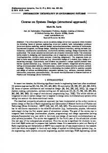
does not reveal the centroid's column coordinate, where X is the x coordinate of the centroid in question, Xmax is the greatest x coordinate of all the centroids, and ncols is the number of columns on the slide. Figures 1 and 2 below show two different instances of the problem. The instances consist of arrays of (x,y) pairs representing the positions of the centroids of the tissue samples on the slides. In each figure, we show two close-ups of troublesome regions. Figure 1a seems to be fairly regular to the eye with well-defined rows and columns, but zooming into the data set (figures 1b and 1c) illustrates problem areas. Figure 1b illustrates problems due to missing points and deviation of points from nice straight columns. Figure 1c illustrates two different problems: two dots lie in what seems to be a missing
2/15/05
Page 2
row (third row from the top) and the correspondence between the bottom rows in the left half and the right half of the image is not clear. There are various reasons why this might happen, ranging from human error to shearing of the paraffin during handling, but this type of shift makes it impossible to know with certainty what is the correct labeling in these areas. The problem of sparse data is also evident in various regions of figure 2a. Figure 2b shows a close-up of the top left hand corner of figure 2a. It is difficult to know the row and column numbers of the points in the top left corner, especially when using an algorithm based on local structure. Finally, figure 2c shows a close-up of the bottom left corner. The problems encountered in labeling the datasets in figures 1 and 2 are detailed in the Results section below. We have developed an algorithm for labeling rows and columns in irregular arrays of dots which robustly handles the irregularities described above. The approach is rather different in spirit from the more usual Bayesian restoration of images [Geman and Geman, 1984] recently applied to similar problems [Hartelius and Carstensen, 2003]. In that technique, a quality of match between the image and a template is optimized. Similar approaches are described in [Amit and Kong, 1996, Chui and Rangarajan, 2000, Zucker et al., 1999, Carstensen, 1996, Cross and Hancock, 1998, Felzenszwalb and Huttenlocher, 2000, Boykov and Huttenlocher, 1999] and usually involve some sort of annealing algorithm for optimizing a global goodness of fit [Salamon et al., 2002]. Our approach is similar to algorithms for automated theorem proving [Robinson, 1963] insofar as it proceeds via a sequence of deductions concerning the lattice structure. At each stage of the algorithm, we work from information assumed correct to a high degree of certainty. The deductions we make are of the form: if a certain centroid is in row n, then the centroid just above it must be in row n+1. We begin from a region that conforms well to our template of a local-lattice structure and spread our labeled region out from this initial seed. In so doing, the algorithm essentially works through a process of structural diffusion. Structural diffusion is a model that has been used in the study of liquid structure [Baer et al. 1995]. The basic idea behind the model is that the local structure in the liquid strongly resembles the regular lattice structure of a solid but that the longer-range structure breaks down and undergoes a distortion in moving from point to point. The process is modeled as a diffusion process in the space of local structures and the parameters of such structures are fit to neutron scattering experiments to characterize the global structure in the liquid. In what follows we make use of this analogy in two ways. First, we associate to each location a local structure, which is a best match to the local configuration -- a point and its .nearest neighbors. Second, our algorithm moves systematically outward from a starting position mimicking a diffusion process. The analogy stops here; the diffusion described below is a diffusion of identification. The Solution a. Locate Starting Point
2/15/05
Page 3
As our first step, the algorithm searches for a good starting region defined as a region of centroids, which is the best match to our template of a regular local lattice. The local lattice that the algorithm uses as its template consists of a three-by-three grid of points representing a center and its eight nearest neighbors. For each point in the input list, the algorithm selects a best local lattice and calculates a measure of the goodness of fit. The points are then sorted by goodness of fit to determine the starting point. The measure we used for the quality of fit at a given lattice site, (xc, yc), was computed as follows. The lattice points relative to the center (xc, yc) are given by (2)
(xgrid , ygrid ) = (xc , yc ) + K ⋅ va + L ⋅ vb
where K and L are integers and va and vb are the two lattice vectors that describe the local lattice and that remain to be selected as part of the fit. Note that va and vb need not be orthogonal vectors. The eight closest centroids N8 ={(xk, yk), k=1,…,8}, are each associated with a node on the model grid by minimizing (3)
(xk − x grid ) 2 + (y k − ygrid )2
over the values of K and L for any given values of va and vb, where (xgrid, ygrid) are as defined in Eq. (2). The grid parameters va and vb are then adjusted to minimize the sum of the squared distances from the actual positions of the eight points closest to (xc, yc) and their nearest lattice sites. Specifically, (4)
8 2 2 Fit(xc, yc) = Min ∑ ((xk − x grid( k ) ) + (yk − ygrid( k ) ) ) va ,v b k =1
The sum of these eight squared distances is the measure of the goodness of a region's local lattice match. Given reasonably close starting values of va and vb, a local optimization can be carried out analytically. The choice of K and L for a given center (xc, yc), neighbor (xk, yk), and lattice vectors va and vb is achieved by expressing the displacement (xk-xc, yk-yc) as a linear combination of va and vb, and rounding the coefficients to the nearest integers. Using these integers Kk and Lk for the (xgrid(k), ygrid(k)) positions, the resulting objective function is quadratic in the four unknowns va = (vax,vay) and vb, = (vbx,vby). Setting the four partial derivatives of the objective function in Eq. (4) equal to zero, gives four linear equations which may be solved for the optimal values of va and vb,. The solution determines the horizontal and vertical vectors that generate the best model grid for the region. The starting values of va and vb are va = ( Xmax/ncols, 0)
2/15/05
and vb = (0, Ymax/nrows).
Page 4
Once a region with a good fit value is found, its va and vb are used as initial values for the next optimization. The previous paragraphs describe how each centroid is assigned an associated pair of lattice vectors va and vb and a Fit value. The starting point for the diffusion is the centroid with the best fit value. It is assigned relative row and column coordinates (I,J)=(0,0) and its lattice vectors are denoted by va* and vb*. b. Diffuse Before proceeding with the diffusion outward from this center, we scan the list of centroids for suspicious points; these points will not be visited during the diffusion. Such suspicious points are identified by either (a) having a Fit value in Eq. 4 above some tolerance ε1, or (b) having a match between the local lattice vectors at the point at the starting center point poorer than tolerance ε2. Labeling these points as suspicious is in keeping with our mandate of assigning coordinates only when there is high confidence in the assignment. The selection of the two tolerances ε1 and ε2 is discussed below in the results section. Once these points have been labeled as suspicious, the diffusion proceeds. At each step of the diffusion, the algorithm selects a centroid (xk,yk) to be used as the next center of a new local lattice and then assigns row and column coordinates to all the points lying sufficiently near to lattice sites of a 5x5 lattice centered at (xk,yk). The new center must fulfill four criteria: (a) it has not been labeled suspicious as described in the previous paragraph (b) it has not been labeled ambiguous as described below (c) it has not been previously used as a center in the algorithm (d) it has been assigned relative row and column coordinates (I,J). Among the points that fulfill these four conditions, we select the next center as the one which lies closest to the starting center (I,J)=(0,0), as shown in figure 3. Figures (4a,b,c) illustrate the diffusion pattern the algorithm generates as it looks for neighbors to label. Note that condition (d) implies that initially only the starting point can be chosen as a center. We denote the coordinates of the next center by (xk,yk) and its assigned relative row and column coordinates by (Ik,Jk). The algorithm proceeds to generate the locations for the 25 grid points (xgrid, ygrid) in the local 5x5 lattice centered at (xk,yk); for each K and L value between –2 and 2, we find the centroid with coordinates (x,y) closest to (xgrid, ygrid ) = (xk , yk ) + Kvak + Lvbk
and tentatively assign it the coordinates
(Inew, J new) = (Ik , Jk ) + (K,L) . These tentatively assigned coordinates are actually assigned to this centroid only if no previous coordinates have been assigned to this point and the distance
2/15/05
Page 5
2
(x − x ) + (y − y ) grid
2
grid
is less than a specified tolerance ε3. If coordinates have previously been assigned and they do not match the newly calculated coordinates, then the centroid is marked as ambiguous and thus will not be used as a center. The diffusion process continues until all eligible dots have been used as the center dot. The algorithm then translates the relative row and column coordinates (I,J) to absolute row and column coordinates (M, N) = (I, J ) − (Imin,J min) + (1,1)
where Imin and Jmin represent the smallest assigned I and J values. Besides the row and column assignments, the output of the algorithm includes lists of suspicious, ambiguous, and unlabeled centroids. c Parameter Settings The algorithm described above requires specified values for three tolerances εi, i=1,2,3. These tolerances specify limiting values of certain quantities calculated from the (x,y) coordinates of the centroids and, as such, are highly dependent on the scale used in digitizing the image. To eliminate this dependence, the values of these three ε’s are calculated from three user specified tolerances δ i, i=1,2,3 which are measured in units of a lattice spacing. This section describes the correspondence between these ε’s and δ’s and specifies precisely how the ε’s are used. To rescale from units of a lattice spacing to the units used in the digitized grid, it is convenient to define a parameter L, which represents the mean lattice spacing1 L=
1 2
va* + vb*
where va* and vb* are the lattice vectors of the best lattice as defined at the end of the Locate Starting Point section. (a) Epsilon 1 ε1 = N nn ( Lδ1)
€
2
where Nnn is the number of nearest neighbors (which our algorithm currently takes as eight). Since ε1 is used in the test
1
It is possible to separate the scales of Δx and Δy but since our application did not require it, we did not do so.
2/15/05
Page 6
ε1 < Fit(xc, yc) and Fit(xc,yc) is a sum of Nnn squared deviations, δ1 represents the average deviation between a grid point and a neighbor point in units of L. (b) Epsilon 2 The second user specified tolerance, δ2 is used to label suspicious points on the grounds that their lattice vectors deviate too much from the ideal. In the algorithm, this is measured by ε2 >
vi vi*
– 1 ; i = a,b.
Since ε2 specifies a fractional difference, we take δ2 =ε2. This makes δ2 a fractional threshold comparing the size of the locally optimized lattice to the best lattice. This test condition serves to eliminate harmonics2. If the optimized lattice is too small, we say that the lattice vectors correspond to higher harmonics; similarly, if the lattice is too large we call it lower harmonics. (c) Epsilon 3 The last user specified tolerance ε3 is used in ε3 >
2
(x − x ) + (y − y ) grid
2
grid
to decide whether the neighbor (x,y) of our local center should be labeled based on its proximity to the nearest grid point emanating from the local center. Defining δ3 by δ3 = ε3 /L makes δ3 scale independent. (d) Experimental values for δ’s 2
If a set of points are well described by the lattice vectors va, vb then they are also well described by va/2 and vb/2. We call these locally optimal solutions harmonics. 2/15/05
Page 7
Table 1 shows the range of parameter values that produced satisfactory performance using our labeling algorithm. The table also summarizes the meaning and use of each of the parameters. Tolerances δ1
Liberal 0.20
Conservative 0.15
δ2
0.30
0.10
δ3
0.25
0.15
Meaning
Use
Mean deviation of neighboring points from the local lattice Fractional deviation of local lattice vectors from best lattice vectors Deviation of one neighbor to nearby grid point
Decide whether to use centroid as center Decide whether to use centroid as center Decide whether to assign label to neighbor
Table 1 Results The algorithm described above performed satisfactorily on all 5 datasets considered. This is admittedly scanty.The team of students working on the project have graduated and Chromavision has moved on to modified forms of the algorithms incorporating trade secrets they are not willing to divulge. The strength of our results is in demonstrating a way to extract local information from global, i.e. to show the viability of an alternative approach to scene analysis problems. The results presented below are sufficient to show the basic strengths and weaknesses of the algorithm. The data shown in figures 1 and 2 were particularly problematic. The troublesome regions of each figure are in the bottom left corner, shown in the close-ups in figures 1c and 2c. The centroids in these regions received labels that depended strongly on the parameters used and therefore served to define the range of reliable values shown in Table 1. To discuss the problems encountered, it is useful to introduce three complementary ways to visualize the results of the algorithm. The first is just the finished version of the lattices generated during the diffusion phase. Figure 5 shows this view of the labeled dataset from figure 1. The left labeling was generated using conservative values of the tuning parameters δ while the right half used liberal values. Below each of the subplots showing all of the centroids is a labeled close-up of the bottom left corner corresponding to figure 1c. For legibility only the labels suspicious (susp), ambiguous (ambg) and unlabeled (unlb) were included in the figure. Note that conservative values for the parameters label fewer points and result in one unlabeled centroid while liberal values tend to overlabel and result in six ambiguously labeled points. The lattice visualization shows each edge (the line segment connecting two adjacent points in a row or column) as represented in six different local lattices. These lattices are well aligned if the six line segments appear as a single line segment. Small misalignments cause the line segment to appear thicker, and large misalignments produce
2/15/05
Page 8
shadows or completely separate traces. As a result, this way of displaying the data explains any difficulties encountered by the algorithm. The ambiguous labels are due to the very slanted local lattice clearly visible in the liberal labeling. This lattice does not show up in the conservative labeling since its center was labeled suspicious and therefore not used to label nearby points according to its local lattice. The second visualization of the labeling is shown in figure 6. Again, the figure shows the result of the conservative and the liberal labelings for the dataset of figure 1. This view shows the grid generated by connecting each centroid to the adjacent centroids in its assigned row and column. This representation displays the global structure resulting from the assignments. The rows and columns can be easily discerned, and deviations from a regular grid shape stand out. Irregularities in the grid pattern identify centroids with questionable assignments. For example, the centroid left unlabeled by the conservative parameter values is seen to lie at a “fault line” where the grid to its left is shifted by about half a grid spacing relative to the grid to its right. In this situation, it is better for the algorithm to focus the attention of the user to this region than to come up with purported labels. Both extremes of parameter values fulfill this goal of pointing out problem areas. The third visualization for this same dataset is shown in figure 7. This graphical representation displays the lines that are the least squares fit to the centroids in each row and in each column. These lines summarize the global structure that has been assembled by the algorithm. Any nonlinear trends or deviations within a row or column are clearly visible within this representation and show the variation of local structures relative to the global structure. The lone pair of centroids in the 5th row from the bottom are very easy to spot in this view. In retrospect it is also easy to spot these two points in the grid representation of figure 6 and represent another reason to call in a human operator. The “fault line” of figure 6 is also evident here in figure 7. All three visual representations make it easy to spot the missing rows and columns. The grid and the lattice representations make clearly visible any misalignment between two intentionally separated regions. Note that figure 5 shows how a region boundary projects the local structure of its region into the missing row or column. A misalignment between the regions will appear as a series of misalignments between the local lattices centered on opposite sides of the missing row or column. Thus, the local structure for the boundary centroids spans the missing row or column and resolves the offset between the regions. Recall that in order to span the gap across missing rows, the diffusion used 5 by 5 lattices to attempt labeling. Our visualization shows only local 3 by 3 lattices to minimize clutter in the image. The sensitivity to parameter values is further illustrated by considering the labelings for the dataset from figure 2 shown in figures 8 (local lattice view), 9 (grid view) and 10 (lines view). Both the conservative and the liberal values for the parameters focus the operator attention on the problem area in the bottom left corner. Again we see that conservative settings leave many points unlabeled, while liberal settings label many points ambiguous. The best results are obtained by taking a conservative approach to
2/15/05
Page 9
allowing centers by keeping the conservative setting δ1=0.15 while allowing liberal labeling of neighbors from approved centers δ3=0.25. The third labeling in figures 8-10 show the results of the mixed setting δ1=0.15, δ2=0.30, and δ3=0.25. This labeling shows that the culprit is the point in the second column which lies a little too far above the fourth row from the bottom.
2/15/05
Page 10
Discussion There are a number of possible extensions to this algorithm. The least squares lines in the third graphical representation can be used to extend the global structure into sparse regions, and enable the assignment of row and column indices to centroids that were left unlabeled by the local structure algorithm. The grid can also be extended across empty regions to connect isolated groups of centroids. Such regions occur, for example, if there are too many consecutive missing rows or columns, so that the lattice cannot reach across the gap. Alternatively, the lattice size could be increased to bridge this gap, but larger lattice sizes will not perform as well when there is significantly deviating local structure. The tolerances used to determine whether to label a centroid could be based on the va and vb of the nearest centroid that has previously been used as a center, rather than basing them on the va and vb of the best lattice. This would allow the local structure to deviate further from the local structure of the best lattice, provided the local structure changes in a sufficiently gradual manner. The closeness of a centroid to the nearest grid intersection could have been used as a fourth measure of the confidence in its row and column assignment. The row and column assignments of centroids that are further from an intersection of the grid may be questionable. Using this measure would enable the algorithm to perform further consistency checks thereby resolving some ambiguities and identifying others. These and other possible extensions would of course incur additional processing costs. Conclusions We presented a robust algorithm for machine labeling of rows and columns in slightly irregular arrays of points. Arrays of samples are used in many areas, for instance 96 well plates, slides for combinatorial chemistry and multi well carriers for synthesizers. In all these cases current design relies on the wells or dots being in predictable positions so they can be processed or read by robotic equipment. If for any reason the positioning is not as expected, the only possible response is to shut down. Augmenting a vision system with this algorithm would allow robotic systems of this type to recover from minor positioning errors. Beyond its possible uses in similar chemical contexts, the algorithm described in the manuscript is an interesting example of extracting global information from local structure. To accomplish this task, the algorithm hierarchically extends the structure from an initial seed where the match to a local template is optimal. It thus adheres to the classic paradigm for extracting global information described for example in [Duda et al. 2001] or [Ballard and Brown 1982]. The present effort represents a novel example of this technique based on structural diffusion. Several graphical representations of the output data were presented. These different representations show complementary aspects of the local and global structure in the data
2/15/05
Page 11
and enable fast visual analysis of any problems that the algorithm needs to bring to the attention of the operator. References Amit, Y., Kong, A. IEEE Pattern Analysis and Machine Intelligence 18:225-235 (1996). Baer, S., Gutman, L., Silbert, S. J. Non-Crystalline Solids 106:192-193 (1995). Ballard, D.H., Brown, C.M., Computer vision (Prentice Hall, Englewood Cliffs, 1982). Boykov, Y., Huttenlocher, D.P. IEEE Conf. Computer Vision and Pattern Recognition, 2:517-523 (1999). Carstensen, J.M. Computer Vision and Image Understanding 63:380-387 (1996). Chui, H., Rangarajan, A. IEEE Conf. Computer Vision and Pattern Recognition, 2:44-51 (2000). Cross, A.D.J., Hancock, E.R. IEEE Pattern Analysis and Machine Intelligence 20:12361252 (1998). Duda, R.O., Hart, P.E., Stork, D.G. Pattern Classification, (J. Wiley, New York, 2001). Felzenszwalb, P.F., Huttenlocher, D.P. IEEE Conf. Computer Vision and Pattern Recognition, 2:66-73 (2000). Geman, G., Geman, D. IEEE Pattern Analysis and Machine Intelligence 6:721-741 (1984). Hartelius, K., Carstensen, J.M. IEEE Pattern Analysis and Machine Intelligence 25:162173 (2003). Robinson, J. A. Journal of the ACM 10:163-174 (1963). Salamon, P., Sibani, P. Frost, R. Facts, Conjectures, and Improvements for Simulated Annealing (SIAM, Philadelphia, 2002). Zucker, S.W., Pelillo, M., Siddiqi, K. IEEE Pattern Analysis and Machine Intelligence 21:1105-1120 (1999).
2/15/05
Page 12
FIGURE CAPTIONS: Figure 1 An example of the arrays of points to be classified showing details of difficult areas. Figure 2 A second example of the arrays of points to be classified, again showing details of difficult areas. Figure 3 This figure illustrates the first two steps of the diffusion process using a 3x3 grid to avoid cluttering the figure. The center (filled circle) of the lattice marked by solid lines is the starting point for the diffusion process. The center of the lattice marked by dashed lines is the second center processed. The points marked by X’s are the eligible centers for the third local lattice. Figure 4 The algorithm proceeds by finding the most regular local lattice and diffusing out from that seed using the local lattice as a guide. The three portions correspond to progressively later times during the algorithm. Figure 5 The dataset from figure 1 at the completion of labeling using both conservative and liberal values of the parameters. In the upper figure, only the unlabeled and ambiguously labeled points are marked by X’s for readability. Note that conservative values for the parameters result in fewer labeled points and result in one unlabeled centroid while liberal values tend to overlabel and result in six ambiguously labeled points. Figure 6 This view of the labeling from figure 5 replaces the local lattice lines by line segments connecting the labeled points. This representation displays the global structure resulting from the assignments. The rows and columns can be easily discerned, and deviations from a regular grid shape stand out. For example, the centroid left unlabeled by the conservative parameter values is seen to lie at a “fault line” where the grid is shifted by about half a grid spacing. Figure 7 The third visualization for the labeled dataset of figures 1, 5 and 6. This graphical representation displays the lines that are the least squares fit to the centroids in each row and in each column. Figure 8 The dataset from figure 2 is shown at the completion of labeling using conservative, liberal, and mixed values of the parameters. Again, conservative values for the parameters result in fewer labeled points while liberal values tend to overlabel. Figure 9 The results for the example in figure 2 are shown in the connected grid points view. Figure 10 The results for the example in figure 2 are shown overlaid by the least squares lines for each row and column.
2/15/05
Page 13
1b 1000
900
800
700
600
500
400
300
200
1c 100
0
0
100
200
300
400
500
600
1a
900 250
200 850
150
800
100
750 210
220
230
240
250
260
270
280
50 50
1b
100
150
1c
Figure 1
200
1800
2b 1600
1400
1200
1000
800
600
400
200
2c 0
0
100
200
300
400
500
600
700
800
900
2a
450 1600 400 1550 350 1500 300 1450 250 1400 200 1350 150 1300 100 1250 50 20
40
60
80
100
120
140
160
50
180
2b
100
150
200
250
2c
Figure 2
300
350
400
Figure 3
1000
1000
900
900
800
800
700
700
600
600
500
500
400
400
300
300
200
200
100
100
0
0
100
200
300
400
500
600
0
0
100
200
300
1000
900
800
700
600
500
400
300
200
100
0
0
100
200
300
Figure 4
400
500
600
400
500
600
1000 1000 900 900 800 800 700 700 600 600
x
500
500 400 400 300 300 200
x x xx x x
200
x
100
x
100
0 0
0
100
200
300
400
500
260
100
200
300
600
220
200 susp
200
susp
180
180
susp
susp
160
160 susp
susp
ambg
140 ambg
120 susp
susp
susp ambg
susp unlb susp
ambg
120
susp
100
100
susp
susp
susp
80 susp
susp
60 50
500
240
220
80
400
260
240
140
0
600
susp ambg
susp ambg
susp
60 100
150
200
Conservative
50
100
150
Liberal
Figure 5
200
1000
1000
900
900
800
800
700
700
600
600
x
500
500
400
400
300
300
200
200
x
x
100
0
0 0
xx x x xx
100
100
200
300
400
500
600
0
260
260
240
240
220
220
200
400
500
600
180
susp
susp
160
ambg
160
susp
140
susp
120
ambg
ambg
susp
120 susp
susp susp unlb
100 susp
susp
80 susp
susp
100
150
susp ambg
100
susp
susp
60 50
300
susp
180
80
200
200 susp
140
100
susp
200
susp
susp ambg
ambg
60 50
100
150
Liberal
Conservative Figure 7
200
x
1600
x
1600
1800
x
1600
1400
1400
1200
1200
1000
1000
800
800
600
600
400
400
x
1400
1200
1000
800
600
400
x x x x x xx xx x x x x
200
0
0
100
200
x x x xx x
200
x x 300
400
500
600
700
800
900
0
0
100
200
x
200
300
400
500
600
700
800
900
0
0
450
450
450
400
400
400
350
350
350
300
300
300
susp
susp
susp
susp unlb
susp unlb
200
200
400
500
susp
600
700
800
ambg
200
susp
200 susp
susp unlb
unlb
unlb
unlb
ambg
150
150 unlb
unlb
unlb
unlb
susp unlb
unlb
unlb
50 50
100
150
200
250
300
Conservative
Figure 8
350
400
ambg
150
ambg
ambg
100
100
900
susp
susp ambg
ambg
susp unlb
300
250
250
250
100
100 susp
50
50 50
100
150
200
250
Liberal
300
350
400
50
100
150
200
250
Mixed
300
350
400
1800
1800
x
1600
1800
1600
x
x
1400
1400
1200
1200
1200
1000
1000
1000
800
800
800
600
600
600
400
400
x xx xx
200
0
-200
0
xxx x x x x x
100
200
400
x xx x x x
200
x x 300
400
500
600
700
800
900
x
1600
1400
0
0
-200
-200
0
100
200
x
200
300
400
500
600
700
800
900
0
450
450
450
400
400
400
350
350
350
300
300
300
susp
susp
susp
250
250 susp unlb
susp unlb
200
100
200
300
400
500
susp
600
700
800
susp
250 susp
susp unlb
ambg
susp
ambg ambg
200
200
susp unlb
susp
unlb
150
ambg
150 unlb
unlb
ambg
150
unlb
100 unlb
unlb
100
susp unlb
unlb
unlb
ambg
ambg
100 unlb
50
susp
50 50
100
900
150
200
250
Conservative
Figure 10
300
350
400
50 50
100
150
200
250
Liberal
300
350
400
50
100
150
200
250
Mixed
300
350
400