collection, display, and analysis of data for distributed autonomous systems. ... As for analyzing the data after it has been collected, a temporal logic is a good ...
A Suite of Tools for Debugging Distributed Autonomous Systems David Kortenkamp1, Reid Simmons2, Tod Milam1, and Joaquín L. Fernández2
1
Metrica Inc./TRACLabs
1012 Hercules Houston TX USA 77058 {korten, tmilam}@traclabs.com
2
School of Computer Science Carnegie Mellon University 5000 Forbes Avenue Pittsburgh, PA 15214 USA {reids, joaquin}@cs.cmu.edu
ABSTRACT
This paper describes a set of tools that enables developers to log and analyze the run-time behavior of autonomous control systems. A feature of the tools is that they can be applied to distributed systems. The logging tools enable developers to instrument C or C++ programs so that data indicating state changes can be logged automatically in a variety of formats. In particular, run-time data from distributed systems can be synchronized into a single relational database. Tools are also provided for visualizing the logged data. Analysis to verify correct program behavior is done using a new interval logic that is described in this paper. The logic enables system engineers to express temporal specifications for the autonomous control program that are then checked against the logged data. The data logging, visualization, and interval logic analysis tools are all fully implemented. Results are given from a NASA distributed autonomous control system application.
1. Introduction Debugging and verifying distributed control programs is notoriously difficult, yet such control programs are becoming more and more common for complex applications. Examples include spacecraft control [Muscettola et al 1998], process control [Bonasso 2001], multiple robot applications [Simmons et al 2000], and production plant control [Musliner and Krebsbach 1998]. In each case, concurrent programs, often on separate computers, generate control commands for single, or multiple, devices. The difficulty in debugging such applications is directly related to their distributed nature. When a problem arises, it is often difficult to isolate the problem to one specific control module due to timing constraints, interprocess communication, and synchronization. The traditional dynamic method for debugging sequential software has no timing constraints. For such systems, cyclic debugging (running the program until an error shows up, examining the program state, inserting assertions, and re-executing the program to obtain additional information) is commonly used [Tsai et al 1996]. However, there are several reasons why this approach cannot be applied to distributed control programs: • Often the distributed processes cannot be paused for examination, since they are controlling physical hardware. • There is no central, global state (or even global clock) to reference state values, which makes it difficult to reason about the “state” of the system at a given time. • Due to latencies and timing issues, distributed control programs are inherently nondeterministic and non-repeatable. Moreover, the types of questions that developers of distributed, autonomous control systems need answered are often temporal in nature and refer to interdependencies between modules. For instance, developers may have questions such as: • Do two states in separate control programs always change together? • What is the latency between the change in one and a change in the other? • When event X occurs in one module, how long before event Y occurs in a second module? Traditionally, such questions are answered by instrumenting programs to write data to files, collecting and collating the files, and inspecting the execution traces to look for patterns of interest. Each phase of this procedure is typically done by hand and is application-specific. Thus, the process tends to be tedious and error prone. Our approach is to develop application-independent tools that are tailored for the collection, display, and analysis of data for distributed autonomous systems. This paper presents a suite of data collection and display tools and a temporal, interval-based logic that facilitate debugging and verifying distributed programs. The data collection tools enable developers to easily instrument control programs and to synchronize the data collected in a distributed system. The display tools enable developers to visually spot trends in the data. The interval logic is used to analyze the logged data to determine
1
whether the execution of a distributed program is consistent with a formal description of the program’s behavior. The logic includes mechanisms to deal with real time and has powerful mechanisms to specify relationships between events, temporal intervals, and sets of these constructs. The data collection, display, and logic tools all work together via a common relational database, which facilitates data storage and retrieval. 1.1.
Overview
Our approach consists of three sets of tools: Tools for instrumenting distributed, real-time systems and logging execution data into a database, tools for doing temporal analysis of execution traces, and tools for visualizing data. The tools are connected through a relational database. Figure 1 shows the general architecture. A library of real-time data collection tools called Rlog is used to instrument each of the distributed processes. The Rlog tools send data corresponding to events (state changes) to a centralized database. After execution, an analysis tool, based on a customized interval temporal checking logic (ITCL), uses the data in the database to verify specifications of the distributed system. Counterexamples produced by the analysis tool can be used to help debug the system. In addition, relationships between the data can be visualized using display tools. The rest of this paper describes each of these pieces in detail, and presents results of using the tools in a distributed autonomous control system developed at NASA. Process
Rules (specifications)
Database (data) Process parser ITCL
DB server
data access
evaluate
Report (test result)
USER
Process
ITCL LOGIC
LOG DATA
Figure 1. General Architecture
2
RLOG
1.2.
Related work
Work on collecting data from real-time programs has resulted in a product from RealTime Innovations Inc. called Stethoscope [Schneider 1995]. Stethoscope allows for data collection, display and modification. However, it is limited to real-time programs running under VxWorks and does not offer support for the kind of high-level, crosssystem debugging that distributed systems require. There are recently developed tools for debugging and verifying parallel systems that are related to our research. For example, ParaGraph [Heath and Etheridge 1991] provides a variety of visualizations of a parallel system. There are also tools for debugging and verifying multi-threaded programs, including tnfview [Kleiman et al 1996]. However, none of these tools can offer the cross-system and high-level debugging and verification support needed by autonomous systems. As for analyzing the data after it has been collected, a temporal logic is a good candidate to define the specifications to check on the execution trace data since it can specify properties of event and state sequences. However, traditional linear-time temporal logic, such as PTL [Gabbay et al 1980] and ITL [Moszkowski 1994] or branching-time, such as CTL [Emerson and Clarke 1982], cannot specify quantitative aspects of time. The concepts of eventuality, fairness, etc. that these languages support are all basically qualitative treatments of time. For example, the expression (p→◊q) can be interpreted in linear-time propositional temporal logic as “Every stimulus p is eventually followed by a reaction q.” However, it is not possible to express “Every event p is followed by a reaction q in the next 4 time units.” To overcome this shortcoming, three different methods are typically used to represent metric time [Tsai et al 1996]. One method is to use explicit clock variables, such as a global clock, and bind a variable to the corresponding time when an event occurs. This approach is used in TPTL [Alur and Henzinger 1990] and XCTL [Harel et al 1990]. Another approach uses bounded temporal operators to restrict the time span between two events. Metric TL [Koymans 1990] is one example of this approach. The third method uses a time function, such as the one used in RTL [Jahanian and Mok 1987]. Most of these logics were designed for model checking and they restrict their language to be able to apply verification methods. However, other logics such as Event-based Realtime Logic (ERL) [Chen et al 1991] and Real-time Interval Logic (RTIL) [Razouk and Gorlik 1989] were developed to yield practical tools for software testers running the system and checking the specifications over the trace data.
2. A Running Example A key goal of this research was to be able to handle complex, real-world distributed systems. To that end, we have tested our logging and analysis tools on an automated, distributed system to control an advanced water recovery system (WRS) at NASA
3
Johnson Space Center. The WRS control system consists of four components. We chose one, the air evaporation system (AES), for this test. The entire WRS system and its controllers are described in [Bonasso 2001]. We introduce the AES here and refer to it throughout the rest of the paper.
2.1.
The Water Recovery System
The AES consists of an evaporation loop of heated air blowing through a wick and a condensing heat exchanger (HX). The wick is integrated with a brine reservoir such that when there is brine in the reservoir, the wick will absorb it. Hot air is blown through the wick, evaporating the brine and filling the air with water vapor. When the hot air passes through the heat exchanger, the water vapor condenses into a tank. When the AES is integrated with the rest of the WRS, a pump is used to flow the condensate to the post processor whenever the level in the condensate tank reaches a certain value. There is also an overflow/brine feed tank to catch any overflow from the wick reservoir. There are weight scales on the overflow tank and on the condensate tank. A manual pump is used to pump the brine back into the reservoir from the overflow tank, which also serves to prime the system for stand-alone testing.
2.2.
Sensors
Starting from the blower, there is a heater with an automatic high-temperature cut-off that heats the air to around 60°C, then the wick, and then the HX. There are 15 thermocouples on the wick, and several around the evaporation loop. Only the heater thermocouple (TC29), wick input (TC10) and HX input (TC27) are used for control, but all are logged. There is a differential pressure sensor across the wick and one across the HX, but these are also only for logging. For control, there is a relative humidity sensor (DW01) in the wick (for drying it out), a mass flow meter (FM07) in the evaporation loop, and a liquid flow meter (FM08) in the HX. Two other temperature sensors associated with the dewpoint sensor and gas flow meter are also only logged. Additionally there are ammeters for the blower (PW01), the heater power (PW02), and power to the devices (PW03 - general power). The wick reservoir has high, mid, and low level switches. There is no direct feedback from the relays used to turn on the blower, heaters, and cooling water solenoid valve. Instead, the power sensors and the flow meters are used as indirect feedback.
2.3.
Control
The main purpose of the control is to start the evaporation process (coolant flowing, blower on, heaters on) whenever the low reservoir switch is on, and to stop the process whenever that switch is off. The heater is actively controlled to maintain air input to the wick at 60°C (the heater element temperature is around 175°C). Monitoring is necessary for air and chiller water flow, wick out temperature, and wick dewpoint. The HX chiller water solenoid valve, which is normally open to allow flow, is closed whenever the AES is shut down, so as not to inordinately lower the temperature of the surrounding tubing.
4
In addition, when integrated with the rest of the WRS, AES operations are augmented to include determining whether the condensate will go to the post processor or be recycled, and whether to flow condensate to the post processor when the RO is in purge. An automated three-way valve determines whether AES condensate goes to the post processor or is rejected back to the feed tank. The AES monitors the state of the RO and the level in the condensate tank to try to flow condensate to the post processor whenever the RO is not flowing water to it. This approach insures a longer duty cycle for the post processor.
3. Data Collection The data collection demands of autonomous control systems range from low-level sensory data and the program’s internal state to high-level goals and state transitions. The data collection routines should be easy to use, flexible, and have minimal impact on the run-time of the system. In particular, in designing our data collection routines we imposed the following requirements: • Data collection must be real time • Distributed data must be synchronized through logging to a database • Data must be collected with flexible sampling rates • Data must easily be grouped into logical sets • Data must be collected conditionally (e.g., allowing data only in certain ranges to be collected, or only when it has changed, or only for certain logical sets) In addition, a primary requirement was ease of use. Our goal was to replicate the flexibility and ease-of-use of the printf facility in C, while allowing for more fine-grained control and for distributed operation. In essence, we have implemented a remote printf capability that is called Rlog. Rlog is a tool that enables developers to instrument their programs and direct the output data to a variety of different locations, including the screen, a file, a remote computer, and a database. As with printf, Rlog can directly handle variables whose types are any of the primitive C data types (character, short, integer, long, floating point, double float, string). More complex data structures can be logged by defining a sequence of these primitives. In addition, Rlog enables developers to specify that, periodically, logged variables whose values have recently changed should be collected, that certain subsets of the variables should, or should not, be logged, and that logging should occur only when the values of variables fall within certain ranges. These capabilities provide an expressive power similar to printf, but with much more flexibility as to when, where, and how to collect the data. A final important requirement was portability. Rlog works on the following platforms: Linux, Solaris, IRIX, and NetBSD. We are currently working on a VxWorks port. As much as possible, the code avoids operating system dependent calls to allow for easy porting to new platforms. While Rlog is geared towards the C/C++ programming language, other programming languages (such as Lisp and Java) can access them through foreign function calls.
5
3.1.
Rlog functions
Rlog is implemented as a set of libraries. The libraries, which all share a common interface, are each specialized for logging output to one type of medium (screen, file, database, etc.). Developers use Rlog by adding calls to the library functions throughout their application programs. The developer indicates which output types are needed and, at run time, the necessary libraries are loaded dynamically (as plug-ins). The Rlog interface is divided into a number of different functionalities. There are setup and cleanup functions, unconditional logging functions, change-only logging, conditional logging, and function entry/exit logging functions. The following subsections present each of these capabilities and describe their functional interfaces. 3.1.1. Setup and cleanup Before using any of the logging functions, Rlog must be initialized. The conceptual model is that there are different output types (screen, file, database, etc.) and which output type(s) are active for a given run can be specified dynamically, at run time. The output types are specified symbolically – for instance, one could be called “debug1” – and a configuration file is used to map between the symbolic name and the location of the associated Rlog library for that output type. The configuration file can also include options that are specific for particular output types (such as the file name to use if logging to a file). 3.1.2.
Unconditional logging
In many instances, one needs to log some aspect of the internal state whenever execution reaches a certain point in the program. For instance, one might want to log the pose (x, y, z, roll, pitch, yaw) of a robot immediately after the pose is calculated, or log the temperature and pressure of a tank immediately before a decision is made about what action to take. The basic logging functions all take a set of variables and output the values of the variables, annotated with a timestamp and the name of the host on which the program is running. The logging functions are all optimized to minimize impact on the user program (see Section 2.5). Sometimes, one cannot collect all the appropriate data at one point in the program, but one still wants to treat the collection of variables as a logical unit. This could be due either to variable scooping (local variables may be inaccessible at certain points in the program) or temporal scooping (for instance, one may want to log aspects of the state both before and after an operation occurs). To accommodate this, Rlog supports the notion of an event, which is simply a logical grouping of logged data. The Rlog functions support selectively enabling and disabling collection of events, and the database output type enables one to access data selectively by event. 3.1.3.
Change-only logging
There are many instances when the developer wants to log a value only when it changes. This capability is useful, for example, when dealing with internal state variables. The idea is to register which variables to track and then to output all changed values
6
periodically. Because true change-only logging would require access to operating system commands, we have instead implemented a matched pair of “register” and “flush” commands. Users can register variables that they want to monitor. Then, whenever the user calls a flush command any registered variables that have changed since the last flush are logged. While not ideal (for instance, any changes that occur between flush commands are not logged), these commands are useful for variables that change infrequently but at well-defined points in the programs. 3.1.4. Conditional logging There are instances when the developer will want to log a value only under certain conditions. For example, only log the tank pressure when it is above 100psi. While users can do this by embedding an Rlog call inside a conditional statement (if-then), we have provided functions that perform this type of computation. The advantage is that the conditional logging functions interact with other Rlog functions in beneficial ways. For instance, if a condition is associated with a change-only variable, that variable gets logged only if it changes and the condition is met. 3.1.5.
Function entry and exit
An important part of debugging distributed programs is knowing whether and when functions have been called and when they have finished executing. In addition to providing a functional interface to facilitate this type of logging, we have developed scripts that will read a C/C++ file and automatically add function entry and exit logging commands to each function in that file. Whenever a function is entered or exited, that function name is automatically logged to the database. If users also want to log the parameters to that function, they can use the Rlog functions described above to do so.
3.2.
Output plug-in modules
Rlog enables users to output the logged information to various media, with various formats. Which output types are active at any one time can be set at run time. The plugin libraries associated with each output type are loaded dynamically. This allows users to change library functions without recompiling their programs. For portability, Rlog uses the GNU Libtool to use dynamically loadable modules (similar to shared libraries) for the output plugins. There are currently four types of output plugins available (additional plugins are easily implemented – details for implementing custom plugins are available on the Rlog web site). The implemented plugins are: • Text plugins, which include screen and file plugins. Text plugins output the logged data in ASCII, using either a format specified in the Rlog command or the default format. • Database plugins, which include two SQL plugins. They differ in the schema used for storing the data in a relational database. The database may reside either on the local machine or a remote machine. More details of the database are given in the next section. • Socket plugins are used to send the logged data to the Rlog server on a remote
7
•
3.3.
machine. The Rlog server handles time stamping the remote data to synchronize distributed processes (see Section 2.4). The TCP plugin uses raw sockets for sending the data. The IPC plugin sends the data using the Carnegie Mellon message-passing package (www.cs.cmu.edu/~IPC). The NULL plugin is used to disable logging. This allows the logging code to remain in the client in case future debugging is needed. The NULL plugin has minimal impact on program performance (see Section 2.5).
Database Logging
One option for storing collected data is an SQL relational database. Using this output type gives the user access to powerful search and retrieval capabilities. We have used MySQL as the database because it is widely available and free (www.mysql.com). Overall, we feel that the use of a standard relational database offers much in terms of portability and flexibility in search and retrieval. Since using SQL is not natural for most users, we have written C/C++ wrappers to insert data into the database and to extract data from the database. In this way, the user of our logging tools does not need to know SQL or anything about the schemas used to represent the logged data. The database schema consists of 12 tables: one for the logged event data and one each for the different data types that Rlog supports. The EventData table assigns a unique identifier to each entry and stores the event name and timestamp for each logging call. The individual data type tables contain the information on the logged variables. These records are tied to the EventData table entry using the Id generated in that table.
3.4.
Distributed logging
By using one of the socket output plugins (see Section 2.2), data from different programs running on different machines can be logged to a central location. The computer at the central location must be running an rlogServer program, which collects all the data on a host computer and sends it to a database (or other location). In this way, data from distributed processes can be collected and synchronized together, in one location. The rlogServer uses the same output plugins as a regular Rlog application. The specific output plugin to use is specified on the command line. To output to a database the database must be on the same machine as rlogServer and the MySQL plugin must be specified. When collecting data generated by different processes on distributed machines, there must be some way to timestamp the data using a common clock. When the rlogServer first receives a data message from a remote computer, it starts a new thread that sends a request to that remote computer for its time offset. It then applies that offset to the received message and all subsequent messages from that remote computer. To account for clock drift, it polls the remote computer every two minutes to update the time offset. If the remote computer gives no response then the timestamp is unchanged. The remote machine must be running an rlogTimeServer, which we developed to determine the offset. This server takes minimal CPU time since it is called very infrequently.
8
Time offsets are calculated based on the formula published in RFC 2030 [Mills 1996]. RFC 2030 claims accuracy to “within a few tens of milliseconds.” The following is the relevant part of RFC 2030 for our purposes: “To calculate the roundtrip delay d and local clock offset t relative to the server, the client sets the transmit timestamp in the request to the time of day according to the client clock in NTP timestamp format. The server copies this field to the originate timestamp in the reply and sets the receive timestamp and transmit timestamp to the time of day according to the server clock in NTP time-stamp format. “When the server reply is received, the client determines a Destination Timestamp variable as the time of arrival according to its clock in NTP timestamp format. The following table summarizes the four timestamps: Timestamp Name
ID
When Generated
Originate Timestamp Receive Timestamp Transmit Timestamp Destination Timestamp
T1 T2 T3 T4
time request sent by client time request received by server time reply sent by server time reply received by client
Then the roundtrip delay d and local clock offset t are defined by: d = (T4 - T1) - (T2 - T3) and t = ((T2 - T1) + (T3 - T4))/2”
3.5.
Rlog performance
We have run some performance measures of the Rlog libraries for the different output types. The platform used for these tests was the following: • CPU: Intel Pentium III @ 800Mhz • Memory: 256 Meg. • OS: RedHat Linux 6.2 • Model: Dell Dimension XPS B800r desktop computer The following table shows the number of seconds it takes to call the basic unconditional rlog function 100 times for each of the different output types that we have implemented. These numbers are an average of 10 sets of 100 calls for all data types and include the initialization and cleanup functions required by Rlog. As one can see, turning off logging (the Null output type) has minimal impact on the run time of the program. Even sending data over the network uses only several tens of milliseconds per call. The MySQL results are with the SQL database running on the same computer as the logging program. If the MySQL database is run remotely then the timings are identical to the TCP results since that is how data is transferred to the remote database. Output Type
Time for 100 rlog Calls
Null
9 milliseconds
9
File
53 milliseconds
Screen
534 milliseconds
TCP
711 milliseconds
IPC
750 milliseconds
MySQL
382 milliseconds
We instrumented the AES control system described in Section 2 using the Rlog tools described here. Fifty sensor and actuator values were logged using change-only logging. These included the thermocouples, power, dewpoint, valves, blowers, heaters, etc. Three days of AES control during July 2001 were logged. [Reid: We need to say something more informative; Was any of the data distributed? How much data? How long did it take the programmer to add in the logging statements? Etc]. In the next section, we describe some simple data visualization tools for looking at logged data. Then, we describe a data analysis tool that was developed and applied to the data.
4. Data visualization People have a great facility for visually detecting patterns in data sets. Such patterns, or deviations from expected patterns, may indicate sources of faults in the system. To aid users in such analysis, we have developed some simple tools, implemented in Java, that retrieve data from a logging database and display the data graphically. The tools automatically analyze the data records to extract the types and names of all variables and events stored in the database (see Figure 2). Users interact with the visualization tools to view selected subsets of the data over time or to plot variable values against one another. The visualization tools support three major types of display: 1) raw data, 2) plotting of values against time, and 3) plotting of two values against one another. The raw data display is just a textual listing of the data values of a variable over time. More useful are plots of the data where one can visualize relationships within, and between, variables. One can plot the value of variables over time, either separately or together. For instance, Figure 3 shows two values plotted against time. From the plots, one can readily detect regularities in the dewpoint data and the discrete change in the thermocouple data. Another useful type of display is to view the values of two variables plotted against each other. This type of plot makes explicit the functional relationships between variables, and enables one to spot anomalies in those relationships. For instance, it is clear from Figure 4 that the relationship between heater power and the thermocouple is very nonlinear. Finally, the data analysis tool (described in the next section) produces counterexamples in the form of intervals of time in which a desired property is found not to hold. We have developed a visualization capability, and integrated it with the data analysis tool, to display such counterexamples graphically. This lets the developer see exactly what the program was doing when a violation occurred. For instance, Figure 5 shows a plot of an
10
interval that has been flagged as containing a violation of one of the logical properties that are being checked. Note that this is still a very preliminary data viewer and that, while visualization is important, the emphasis in this project has not been on visualization. In particular, we hope to make use of the results from other researchers to further this aspect of the project.
Figure 2. List of items from the database that can be viewed.
Figure 3. Two variables plotted against time.
11
Figure 4. Two variables plotted against each other.
Figure 5. Plotting an interval in which an error is suspected
5. Interval Temporal Checking Logic (ITCL) Once the data has been collected, we want to analyze it to verify program correctness. We present a real-time interval logic that is used to specify desired properties about the behavior of real-time distributed programs. We also describe a tool that we have developed to analyze a logged execution trace to determine whether it is consistent with the formal specification. When we began this project, we anticipated developing an analysis tool for an existing temporal logic. However, as we surveyed related work (see Section 2) it became clear that no existing logic had the combination of features and usability that we desired. In
12
particular, we wanted a more intuitive logic, since our work is intended to yield practical tools for software testers. This led us to develop a new logic called Interval Temporal Checking Logic (ITCL), which enables concise specification of simple concepts but also has the expressiveness to handle very sophisticated temporal relationships, both qualitative and quantitative. ITCL borrows concepts from both RTL [Jahanian and Mok 1987] and RTIL [Razouk and Gorlik 1989]. From RTL, we adopt the idea that time passes between events, where events are instantaneous, as opposed to many transition systems in which the states are temporal and transitions are instantaneous. From RTIL, we adopt the idea of constructing intervals from time points that may, or may not, correspond to actual events. We also adopt some powerful interval construction operators and the ability to index into sets of entities. Because our focus is on practical validation of executing programs, ITCL adds new operators that facilitate the expression of complex timing and relational properties inherent in real-time distributed software. In particular, we include operators to handle sets of intervals, events, and timestamped values.
5.1.
Basic concepts
While temporal logic provides good low-level mechanisms for expressing sequences of events, reasoning about repeated behaviors over an entire computation is often awkward. Given our interest in checking and debugging program executions, ITCL includes as basic concepts time points, events (representing actions and changes in system status), intervals that are composed of time points and events, and sets of these entities. Having time points, events, and intervals as basic concepts in the logic allows us to define timing and relational properties in a straightforward way. Having sets of these entities as basic concepts allows us to concisely specify global invariants and periodic behaviors over a complete execution. 5.1.1.
Time points, events, and values
Time points are the basic primitives in ITCL. A time point (φ) is an object with an associated real-valued time (time(φ) ∈ ℜ). A time point can be defined as an absolute point (e.g., noon on January 3, 2003) or in relationship to other time points (e.g., 5 seconds after some event occurs). An event (ω) is a time point that has additional information, including the type of the event and the values of variables associated with the event. Each log entry in the trace file defines an event. Log entries record relevant changes to the system, including the start and end of significant actions, changes to state variables, and perceived changes in the environment. A value (ψ) is a time point that has an associated value (our implementation of ITCL supports numeric, Boolean, and string values). Values can be derived from events. For instance, if φf is the event signifying that the flow of a pipe changes, then φf.flow is the value representing the rate of that flow at the time the event occurs. Similarly, (5 + φf.flow) is the value representing 5 units plus the flow at the time that φ occurs.
13
5.1.2.
Intervals
Intervals (γ) are defined in terms of a pair of time points (φstart and φend). The semantics are that the interval is closed on the left and open on the right (i.e., [φstart, φ end)). Therefore, the starting and ending time points must be distinct (as a result, ITCL cannot represent single-point intervals). Given an interval γ, ↑γ represents φstart and ↓γ represents φend. The duration of the interval is given by duration(γ) = time(↓γ) – time(↑γ). Often, the start and end time points of intervals are associated with events. For instance, if φSA is an event that signals the start of action A and φEA is an event that ends the same occurrence of A then the interval composed of φSA and φEA represents the time during which that instance of action A occurs. In addition, we consider the whole trace itself to be a distinct interval. 5.1.3.
Sets
While time points, events, values, and intervals are useful concepts, we need to refer to sets of these concepts in order to represent and reason about behaviors of programs over whole executions. ITCL allows any of the basic concepts to be aggregated into sets of similar concepts. An event set (Ω) aggregates events of a given type in a trace file. For example, if we have an event type start_A then we can define an event set that corresponds to all the times that action A began execution. Event sets can also be defined as Boolean combinations of other event sets (union, difference, etc.) and as conditional filters (e.g., all events of some type occurring within a given time window, or all events whose associated variable values exceed a given threshold). Section 5.2 describes how event sets can be defined in ITCL. Time point sets (Φ) can be derived from event sets. For example, one can define a time point set corresponding to the event set start_A, which represents the time points at which those events occurred. From this set, we can create a new time point set representing the time points five seconds after the start_A events occur. We might need such a set, for instance, to specify that no event of some other type occurs within five seconds after any start_A event occurs. Finally, interval sets (Γ) can be defined in many ways, including defining them from individual intervals, from pairs of time point sets, or from relationships between events (see Section 5.2). Interval sets enable us to specify global or periodic properties over the complete program execution, or some subset of it. Time point sets (similarly for event sets and value sets) have an implied ordering of their elements, based on their times of occurrence (for points with the same timestamp, some canonical ordering is chosen, such as lexigraphically by event type). Thus, we can index sets, so that Φ[i] is the ith element of the set, according to the ordering.
14
γi.j γ1.1
ω1.1 φ1.1
φ5.1
γ1.2
γ2.1
ω1.2 φ1.2
ω4.1 φ4.1
φ5.2
ω1.i φ1. i
Event set Ω1 = {ω1.1, ω1.1, …} Time point set Φ1 = {φ1.1, φ1.2, …} Interval set Γ1 = {γ1.1, γ1.2, …} Figure 6. Events, event sets, time points, time point sets, intervals and interval sets.
Figure 6 shows several events, time points, intervals, and associated sets. Note that we use two indexes to denote items in a set. The first index represents the set (based o0n the type element) and the second represents the order of the item in the set. For example, φ5.1 represents the first item of time point set Φ5.
5.2.
ITCL Syntax and Semantics
This section describes the syntax and semantics of ITCL for defining basic concepts (time points, events, values, intervals, and sets), and for defining specifications that can be checked against trace files. To facilitate the twin goals of concise specification of simple concepts and support for specification of sophisticated concepts, ITCL has many ways for defining each of these basic concepts. 5.2.1.
Defining time points, events, and values
As described previously, a time point can be defined by an absolute time (real number) or by an event or value (both of which are types of time points). For an interval γ, ↑γ and ↓γ represent the start and end time points of the interval, respectively. The “extension” operators, φ→t and t←φ, represent the time points t time units after φ and t time units before φ, respectively. Formally, time(φ→t) = time(φ) + t and time(t←φ) = time(φ) - t. Events can be defined in only one way – with respect to entries in a trace file. In particular, event sets are defined simply by providing the name of the event type. Individual events are defined by indexing into event sets, as described in Section 5.1.3. A values can be defined from a constant (e.g., 5 or “green”) or by a variable associated with an event (φ.var). For instance, in one of our test programs, the event type train1cv is logged whenever a state variable associated with train train1 changes value. The value of the speed variable for the train1cv event is then referred to as train1cv.speed (technically, since train1cv specifies an event set, train1cv.speed actually defines a value set).
15
Arithmetic operations (+, -, *, /) and relations (, ≥, =, ≠) can be used to define new values. These work in the obvious way. For instance, if ψ1 and ψ2 are numeric values then (ψ1 + ψ2) is a numeric value as well. Values and constants can be combined (e.g., ψ+5), since a value can be defined from a constant. The timestamp of a value created from a constant is the time of the start of the execution trace. The timestamp of a value that results from an operation between two other values is the timestamp of the later value: time(ψ1 op ψ2) = max(time(ψ1), time(ψ2)). 5.2.2.
Defining intervals
Intervals in ITCL are defined using the "search" operators φ⇒T (search forward) and T⇐φ (search backward), where φ is referred to as the start point, and T is either a time point or time point set. If T is a time point, the search operator defines an interval composed of the two points: φ1⇒ φ2 ≡ [φ1, φ2), time(φ1) < time(φ2) ⊥, otherwise φ2⇐ φ1 ≡ [φ2, φ1), time(φ2) < time(φ1) ⊥, otherwise where ⊥ is the undefined interval, which indicates that there is no interval for which the definition holds. If T is a time point set, the idea is to search for the closest time point in the set that occurs strictly after (before) the start point. φ1⇒ Φ ≡ [φ1, φi), ∃ 0≤i 1)) }; ####### is FALSE because: When it2_1 has the value: Intervalvar= Start: sec = 996622397 usec = 137780 End: sec = 996622428 usec = 447794 the condition (forall) becomes false Operation ALWAYS is FALSE. BECAUSE: CONDITION doesn't hold at the beginning of interval: sec = 996622397 usec = 137780 ####### # First it is false because, initially, the switch*State has no value. # Then it is false because of the delay. # We can also consider some delay T1: T1 = 2; with_delay = start(main_and_bl_on)~>T1 ->end(main_and_bl_on); # This is in case T1 is greater than the interval where pw is on with_delay = with_delay && main_and_bl_on; forall it2_1: with_delay { during it2_1 always ((RLogChangedValue.FlowMeter07 > 1)) }; # After turn on the blower power and the general power, # the FlowMeter07 must return readings greater than 1 # and the FlowMeter08 between 7 and 8 main_and_bl_on = [( RLogChangedValue.Switch3State == 1) && ( RLogChangedValue.Switch1State == 1) ]; forall it2_1: main_and_bl_on { during it2_1 always ((RLogChangedValue.FlowMeter07 > 1) && (RLogChangedValue.FlowMeter08 > 7) && (RLogChangedValue.FlowMeter08 < 8)) }; ####### is FALSE because: When it2_1 has the value: Intervalvar= Start: sec = 996622397 usec = 137780 End: sec = 996622428 usec = 447794 the condition (forall) becomes false
29
Operation ALWAYS is FALSE. BECAUSE: CONDITION doesn't hold at the beginning of interval: sec = 996622397 usec = 137780 ####### # We can also consider some delay T1: T1 = 2; with_delay = start(main_and_bl_on)~>T1 ->end(main_and_bl_on); # This is in case T1 is greater than the interval where pw is on with_delay = with_delay && main_and_bl_on; forall it2_1: with_delay { during it2_1 always ((RLogChangedValue.FlowMeter07 > 1) && (RLogChangedValue.FlowMeter08 > 7) && (RLogChangedValue.FlowMeter08 < 8)) }; # Value of DewPoint1 has to be between 83 and 93 during -> always ((RLogChangedValue.DewPoint1 = 83)); # Temperature of TC10 cannot be greater than 60 during -> always (RLogChangedValue.Thermocouple10 always (RLogChangedValue.Thermocouple11 always (RLogChangedValue.Thermocouple29