A Superparticle Filter for Lane Detection - Semantic Scholar

A Superparticle Filter for Lane Detection Bok-Suk Shin, Junli Tao, Reinhard Klette Department of Computer Science,The University of Auckland, New Zealand

Abstract We extend previously defined particle filters for lane detection by using a more general lane model supporting the use of two independent particle filters for detecting left and right lane borders separately, by combining multiple particles, traditionally used for identifying a winning particle in one image row, into one superparticle, and by using local linear regression for adjusting detected border points. The combination of multiple particles makes it possible to extend the traditional emphasis of particle-filter-based lane detectors (on identifying sequences of isolated border points) towards a local approximation of lane borders by polygonal or smooth curves further detailed in our local linear regression. The paper shows by experimental studies that results, obtained by the proposed novel lane detection procedure, improve compared to previously achieved particle-filter-based results especially for challenging lane detection situations. The presentation of several methods for comparative performance evaluation is another contribution of this paper. Keywords: Lane model, lane detection, lane tracking, particle filter, performance evaluation 1. Introduction Lane detection, lane tracking, or lane departure warning have been the earliest components of vision-based driver-assistance systems. They have been designed and implemented for situations defined by good viewing conditions and clear lane markings on highways. Since those early days in the 1990s, visual lane analysis remains an ongoing research subject [26], with a focus on particular subjects such as accuracy for selected challenging conditions, robustness for a wide range of scenarios, time efficiency, or integration into higher-order tasks. Preprint submitted to Elsevier

October 11, 2014

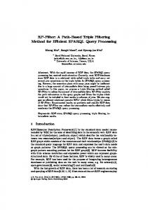
Figure 1: Left: Three examples for data provided by [7] when applying the lane detector described in this paper which produces sequences of individual points. Right: Example when approximating lane borders by line segments [29] for simple data as in Set 3 of [10].

In a general sense, a lane L is defined by sufficient width for driving a road vehicle; it is the space between a left and a right lane border, being arcs γL and γR respectively on a 2D manifold that is not just a plane in general. Many different models have been used for defining lanes (e.g. analytically defined smooth or polygonal curves or sequences of individual border points following some kind of systematic pattern). Figure 1 illustrates on the left (three images) results of our single-lane detector which calculates individual (but locally smoothed) border points using test data provided by [7], and on the right a Hough-transform-based multi-lane detector for road situations defined by straight borders using test data provided in Set 3 of EISATS [10]. This paper discusses basically single-lane detection only, for the lane currently driven by the ego-vehicle (i.e. the vehicle the vision system is operating in), with temporary considerations of multi-lane cases while changing lanes. Contributions of this Paper This paper addresses particle-filterbased lane detectors as described, for example, in [14, 15, 31] that calculate sequences of isolated points for estimating lane borders; these detectors use a generic lane model and they are in particular designed for more challenging input situations such as suburban roads, countryside roads, inner-city roads where a lane border may be defined by parking cars, a change in surface texture (e.g. unpaved road and lawn), and so forth. First, we provide a more general model of a lane also including greater variations in appearances. This adds more flexibility to the used lane model for supporting improved robustness of the resulting lane detector. Second, we modify previously defined particle-filter based approaches (as in the papers cited above) which define particle filters for individual image rows. We use results of multiple particle filters, combine those (also using

2

temporal propagation) into a single particle filter, and call the combined particles now superparticles. The method is proposed for improving robustness for several difficult scenarios. Third, we use those resulting superparticles for ensuring local smoothness of detected lane borders. Finally, we comparatively evaluate our method (against the method published in [14, 15]) for situations when 1. crossing a wide road intersection where no lane markers are visible at all in several subsequent frames (see Fig. 1, two images on the left), 2. varying shadows on the road may be confused with lane borders, 3. changes in lane width or merging lanes require a high flexibility in adapting lane parameters, 4. noisy lane borders make visual lane detections very challenging, or 5. a rainy day creates particular visibility difficulties. We consider the presentation of various options for a comparative evaluation of lane detectors as a further contribution of this paper. By considering the stated selection of challenging scenarios in our experiments we demonstrate the ability of the proposed model, superparticles, and local smoothing to avoid the inheritance of errors; we can show that the proposed technique ensures robustness for various challenging situations. Alternative Approaches and Comparative Evaluations Particle filters are a very common optimisation approach [18]; we improve the generic lane model initiated in [31], and used in algorithms proposed in [14, 15]. Different lane models and particle filters have been used for visual lane analysis, for example, in [4, 9, 20, 22, 25]. Particles used in these papers model also specific road geometry or multi-lane situations; implementations are not available for direct experimental comparisons. Paper [15] already compares the particle-filter-based lane detector (proposed in this paper) with two non-particle-filter-based lane detectors described in [2] and [25]. Experimental results are reported in [15] for various situations and long video sequences by providing “typical results” and statistical data. The paper concludes that the particle-filter-based method of [14, 15] “is comparable with” the method proposed in [2] “based on the overall performance, even a bit better, and more robust than” the method proposed in [25] “for dealing with difficult road situations.” We do not repeat such a study here. 3

There is not yet any satisfying automatic evaluation available for quantifying the performance of a lane detector. For example, we could claim that “lane borders are correctly detected if they are within an error of at most 5 cm to the true lane border”. Between what minimum and maximum distance to the car? What exactly is the “true lane border”? How to measure for cases as illustrated in Fig. 1, left, with missing lane markers? There is also no web-based benchmarking system of reasonable complexity available for lane detection on subsequent frames, which would be appropriate such that authors can compare their implementations themselves (as already common for other subjects in computer vision such as stereo vision or optical flow calculation). Such a benchmark dataset should provide adequate ground truth for lane-analysis tasks. Existing performance evaluations have been done based on different datasets, prohibiting a fair performance comparison. KITTI1 started recently to provide 289 frames with manually labelled frames for evaluating road detection or lane areas. These are isolated frames, not sequences of subsequent frames, and thus not usable for evaluations of dynamic lane detectors as the one proposed in this paper. Besides requiring subsequent frames for evaluating a method using dynamic (temporal) propagation, experiments should also be performed on “long” challenging sequences. For this paper we used four test sequences for which the total number of frames is above 1000. Solved? Lane detection is sometimes characterised as being “solved”. Can we really claim that something, which is non-trivial by nature, is “solved” knowing about all the surprises (e.g. unpaved roads, underground road intersections, or very wide road intersections without any lane marking) which may occur in the real world? The characterization “solved” is only appropriate for about, say, 90% of scenarios while driving in a country with very-well developed road infrastructure, also assuming that lane markings, lane geometry, and visibility conditions are “reasonable” (e.g. for highways or other roads with clearly marked lane borders under good daylight conditions). Detecting the borders of weakly marked lanes, as they often appear in inner-city and rural environments, remains often an unsolved problem due to the high variability in such scene conditions [11]. Current research also considers the subject of lane detection as an integral part of higher-order tasks, e.g. combined with components such as curb detection, traffic sign 1

See www.cvlibs.net/datasets/kitti/eval_road.php

4

recognition, vehicle tracking, visual navigation, and so forth [26]. Lane-Detection Module in a Context The authors do not believe that it is possible to include all the possible contributions for a given road scene (road geometry, lighting, traffic density, weather, road obstacles, pedestrians, occlusions by vehicles, expected velocity, and so forth) into one particular model for lane detection. We rather suggest to include one clearlyfocused lane module into a higher-order driver-assistance system composed of multiple clearly task-focused modules (e.g. one for road geometry analysis, one for pedestrian detection, and so forth). For that reason we decided to focus on an improvement of the generic lane model as initiated in [31]. Which Basic Features? The discussed generic lane model is based on extracting one type of features from an image, namely edges only. There are suggestions for using multiple features, combined with learning, for optimising detection; see, e.g., [12, 13, 27]. This might possibly lead to improvements, still to be verified (e.g. based on future web-based benchmarking data). For example, monocular vehicle detection can benefit from designing a multi-feature-based detector (combining horizontal lines, corners, visual symmetry, and Haar-features), as studied in [24]. However, the authors cannot yet see a proven indication in previously published papers in the “multifeature lane detection” area which other features (alternatively to edges) could possibly become a generic and powerful “companion” to edge features for lane detection. Structure of this Paper Section 2 informs about the basic image processing tasks to be performed for being able to define weights for our superparticle filter. Section 3 outlines the improved lane model and our detector. Section 4 provides a comparative performance analysis between a previous particle-filter-based lane detector and our novel superparticle-based detector. Section 5 concludes. 2. Low-Level Image Processing We follow pre-processing steps as in [14, 15, 31]. We discuss limitations of the used distance properties. Bird’s-Eye View, Vertical Edges, and Oriented Distances For starting the lane detection process, each input image I is warped into a bird’seye view image. In a bird’s-eye view image, lane borders are expected to be 5

roughly parallel, which benefits the lane-detection procedure. To obtain a bird’s-eye view image, some methods require camera focal length and external parameters (e.g. mounting angle) information, others [8, 14] use simply an existing or assumed rectangular planar pattern in the real world to calculate the required homography. For our method it is not important which way is chosen for calculating a bird’s-eye view. In our experiments we adopted the four-points warp-perspective mapping method which proved to be of satisfying accuracy for a large diversity of input data. We calculate an edge map for the bird’s-eye view image aiming at vertical edges rather than horizontal edges. After binarization of the resulting edge map, an oriented distance transform (ODT) is applied for assigning horizontal distance data with respect to detected edge pixels. The resulting distance map allows us to design a novel initialisation method (according to our change of the used lane model) for finding initial border points, used for initialising the proposed superparticle filter. Bird’s-eye View Mapping The perspective input image I is easily mapped into a bird’s-eye view I b using a homography defined by four vertices of a (supposed to be) rectangle in the bird’s-eye view. A four-point correspondence is then used for mapping the input image into a bird’s-eye image. This assumes a planar ground manifold in front of the ego-vehicle for the chosen frame (somewhere in the video sequence) to be used for calculating the homography. We specify in one recorded image four points assumed to be corners of a rectangle; see Fig. 2. (These points could also be marked as a real rectangle in an input scene at the start of a recording.) One image is sufficient for calibrating the homography for the intended mapping into a bird’s-eye view image.

Figure 2: Input image and projected image by WPM.

6

Let pi = (xi , yi , f ), i = 1, . . . , 4, be the four corners in I, for focal distance f . They are projections of four points Pi = (Xi , 0, Zi ) in the ground plane, assuming Y = 0. We have an one-to-one mapping between pi and unknown points Pi , but know that points Pi form a rectangle, which constraints the coordinates Xi and Zi . Altogether, this defines a homography H·p=P

(1)

for mapping all image points p = (x, y, f ) into ground-plane points P = (X, 0, Z). There will be distortions if a pixel at p is actually not showing a point in the ground plane. If using points as shown in Fig. 2, the Euclidean distance d2 (P1 , P2 ) = d2 (P3 , P4 ) (in pixels) can be used as an initial value for the expected width of a lane. A benefit of the described procedure is that the used distance scale in the bird’s-eye view image can be adjusted by selecting different sets of four corners of rectangles. This proved to be useful when detecting discontinuous lane markers as well as for adjusting forward looking situations. A lane in the bird’s-eye image has approximately a constant width, and this is used in the vertical edge-detection procedure. Vertical Edge Detection We adapt an edge detection method, as introduced in [6, 30] for lane detection. Vertical lane-mark-like step-edges in the bird’s-eye image are detected by using magnitudes of approximate derivatives in x-direction only. Those magnitudes are binarized. We remove small segments (considered to be noise) in the obtained binary edge map. Oriented Distance Transform The Euclidean distance transform, applied to the generated binary edge map J, labels each pixel with the Euclidean distance to the nearest edge pixel. Let J(q) = 0 (shown as black pixel) if we detected an edge pixel at p ∈ Ω, where Ω is the set of all pixels. Distance values d(p) = min{d2 (p, q) : J(q) = 0} (2) q∈Ω

are defined by an x- or row-component (x1 −x2 ) and a y- or column-component (y1 − y2 ) in the usual Euclidean distance p (3) d2 (p, q) = (x1 − x2 )2 + (y1 − y2 )2 The row-component defines the oriented distance transform (ODT) which labels each pixel with a distance value to the nearest edge point in horizontal 7

Figure 3: Ideal distance map (top). Incorrect distance map due to noise or a missing edge.

or row direction. Moreover, the values (x1 − x2 ) of the ODT are signed, with a positive value indicating that the nearest edge point lies to the right, and a negative value if it is to the left. Discussion of the ODT The ODT of the edge map offers various benefits. Generally, as a distance transform, every pixel value in the ODT map indicates the column of a nearest edge point. Pixels with an ODT value equals zero can be tested for being lane border points. Lane centre lines are assumed to occur at pixels that have a local maximum in absolute values in the ODT distance map; more specific, at a pixel on a centre line, a positive and a negative value “meet” at adjacent pixels. This information is useful to evaluate potential lane border or centre line pixels when detecting or tracking lanes; see, for example, [15]. However, distance transforms are sensitive to occurrences of noisy pixels. A centre line is also incorrectly located at incorrect coordinate when lane

Figure 4: Multiple lanes with large gaps in lane markings (left), and the resulting ODT map with indicated “issues” caused by missing edges.

8

border disappeared. Figure 3 illustrates sketches, on top for an ideal ODT map in one row (the edges on both sides are labelled by value 0, and the centre point by the appearance of adjacent positive and negative values), and below for a case where one side does not exist (as expected) or is defined by noise; in this case the centre point is shifted to the left or right, also identified by an incorrect distance value. Missing Lane Markers Figure 4 illustrates how (here: missing) edge points of a lane influence the ODT values of surrounding pixels. The missing lane markers in the bird’s-eye view image are denoted by blue dashed boxes. The green lines in the right image are the detected centre lines defined by adjacent negative and positive ODT values (i.e. by pairs of −η and η values); the white lines are detected edges. The yellow dashed ellipses highlight locations of incorrect centre lines (shifts to the left or right, or even splits into several centre lines), caused by the missing lane markers. Therefore, centre lines are not reliable sources for lane detection in cases of missing lane markers, and this was not yet properly considered in the model initiated in [31]. For dealing with this issue, we introduce weights whose values reflect the actual potential contribution to the decision process. 3. Improved Lane Model and Superparticles We improve the lane model of [31] and use it for particle filters for single image rows; due to the modified model this also already represents a modification of the algorithm proposed in [14, 15]. By combining those single-row particles for multiple rows within a temporal propagation of results, we create superparticles. Our concept of temporal propagation aims at reducing error propagation (i.e. the combination of single-row particles is not simply a static, single-frame combination of isolated results, but a dynamic approach resulting in optimised detections in subsequent frames). Modified Lane Model By modifying the model as proposed and used in [15, 31], we model a row in a single lane not only by four but now by five parameters. These parameters identify the pair of lane borders in the ground manifold in one image row. See Fig. 5. Let pl be the point on the left lane border, and pr the point on the right lane border. For simplicity we identify both with their x-coordinates having the current image row identified by a y-coordinate. In the ideal model case, point pc = (xc , y) is the centre point half-way 9

Figure 5: Lane model with parameters pc , αl , αr , βl , and βr ; bold lines indicate lane borders.

between pl and pr , also just identified by a coordinate xc in the current row y. Let h be a fixed positive value. Point pc and height h define an angle α to pl and pr , and angle 2α would define the width of the lane in the ideal case. However, due to the varying distance issues to the centre line illustrated in Fig. 4, we change the model as used in [15] (which uses a constant angle α for both sides of the lane) now to a model where we may have two different angles αl and αr to the left or right. In the particle filter, these will be random angles. These angles define distances ϕl1 and ϕr1 . As h is a fixed value, ϕl1 and ϕr1 are defined by the two α-angles. Angles βl and βr specify the slopes of tangents to the lane borders at points pl and pr , respectively, in the bird’s-eye view image relatively to row y. These angles help to predict the continuity of lane borders. The important point here is: we do not simply create one 5D particle space; rather we consider two separate 4D particle spaces, one independently for each side of the lane. By applying this model, we overcome difficulties of the model used in [15] for cases where lane borders disappear, the lane changes its width, or cases where lane borders are not parallel, e.g. caused by using four points for calibrating the homography H which are not exactly corners of a rectangle. Individual Point Detection Meets Curve Detection As a further model modification, we also use the assumption that lane borders form typically locally straight line segments or segments of smooth curves. The particle filter is in general based on the assumption that lane borders are not defined globally by polygonal or smooth curves; with our new approach we establish a compromise between both classes of techniques. Figure 6 illustrates the improved lane model for one bottom-up propa10

Figure 6: Compromising between parallel borders and smooth curves. Left: Lane model which uses a constant angle α for both sides of the lane, not considering the detection of a smooth curve. Right: New lane model which uses two different angles αl and αr to the left or right, being able to follow smooth curves individually on each border.

gation step in one frame, from row yn to row yn+1 . Constant angles α on both sides (though they may change from yn to row yn+1 ) favour parallel lane borders due to the built-in propagation mechanism in the particle filter, illustrated in the figure by a case where the left local window is on a lane border, but the right window is off. The new model, illustrated on the right, is able to adapt to different curves, individually on each side. Particle Filters In this paper, we apply multiple particle filters based on our new lane model. When assuming that αl = αr then particle filters use 4-dimensional state vectors v = (pc , α, βl , βr ). These state vectors are used for tracking a pair of left pl and right pr border points of lanes. For example, see also lane detection and tracking in [19, 21]. We propose to detect and track a pair of lane border points by propagated particles independently on the left and right, bottom-up in the image. The left border point pl is observed by particles with state vector vl = (pc , αl , βl , βr ), and the right border point pr by particles with state vector vr = (pc , αr , βl , βr ). Again, both filters use 4-dimensional state vectors. Propagating Row Filters through one Frame We detect lane borders not in every image row y; we may use increments 4 > 1 between subsequent rows. Let yn be the nth row considered in the propagation process for one image, for 0 ≤ n ≤ N . The pair (pln , prn ) of two lane borders is determined based on observing two particles vˆln , vˆrn , with predicted values

11

veln , vern . A pair (pln , prn ) propagates particles into the next row yn+1 by specifying pcn+1 first. Let g be the number of generated particles; the number g of particles is generated randomly, assuming a chosen Gaussian distribution. For details of a particle filter (i.e. particle space, dynamic model, observation model, definition of weights, condensation algorithm for re-sampling, and final maximumlikelihood rule, see, for example, [18]). Lane Border Tracking When going from Frame t to Frame t + 1, lane borders of Frame t are seen partially again in Frame t + 1. We assume a forward-driving ego-vehicle with a minor change in driving direction between Frame t and Frame t + 1. Lane border points detected in Frame t which are close to the lower image border disappear, those further up stay in Frame t + 1 but move down in the image (and their actual positions need to be corrected), and we also need to detect a few more new lane border points further up to those which remained from Frame t. Formally, say M ≤ N rows of Frame t are replicated in Frame t + 1, and a remaining number of N − M rows needs to be processed with the newly available data in Frame t + 1. Parameter M is defined by M = N − ut , where ut is determined by the driven distance between times t and t + 1, to be estimated based on the current speed of the ego-vehicle,2 or, if requiring a higher accuracy, based on some visual odometry technique. For example, when driving at about 50 km/h then u = 2 can be used as a rough estimate. For updating the replicated M left or right lane border points, and for processing the remaining N − M new rows, we apply multiple-row particle filters in the considered image rows in a bottom-up approach in Frame t + 1. These multiple-row particle filters consider (in a bottom-up approach in the image) at each processed image row also a few of the previous rows for stabilising the current state. The forwarded M lane border points are applied in the propagation procedure as previous states at the time when the multiple-row particle filter starts. Multiple Particle Filters We extend the single-row particle filters to multiple-row particle filters. When refining particles for Frame t + 1 based on Frame t, this creates a dynamic dependency between particles in (say, g) subsequent image rows. 2

Modern cars support reading of speed and yaw rate.

12

The winning particle vˆn , out of g generated particles, is chosen due to particle weights during the re-sampling process. The particle with the highest weight contributes to the determination of a border point by iterative processing for 0 ≤ n ≤ N . The single-row method for finding a border point, as used in previous publications when applying a particle filter for lane detection, relies very much on the chosen centre point pc and its weight. In cases when an incorrect state is propagated from the previous row to the current row, this critically “infects” the next steps (a case of error propagation) and causes unstable results. In our method, we use the expected local continuation of a lane border, either on the left or on the right, individually. A winning particle is produced by considering not only a few of the previous states (or rows) but also a few steps ahead in the propagation procedure (as a dynamic optimisation procedure). These previous and future states (of a traditional single-row particle filter) define now components of a superparticle, and a superparticle is represented by a combined state vector V. Observations are based on previous and future states for a decision about the current state vector. We prevent errors of single-row particles by considering missing edges, intensity changes, and so forth. Let Vn be the superparticle determined by observed particles in multiple rows, formally represented as follows: Vln = (pc , αl , βl , βr , Vln )

(4)

Vrn = (pc , αr , βl , βr , Vrn )

(5)

Vn = {ˆ vn− , ..., vˆn+⊕ }

(6)

where is the number of backward steps, and ⊕ the number of forward steps. Figure 7 illustrates our combined superparticle filter. Enforcing Local Consistency By the described multiple-particle e filtering, we obtain a predicted particle V . For the xy-coordinates of observed points Vn , denoted by {(x1 , y1 ), ..., (xk , yk )}, we perform a linear regression for fitting a straight line y = ax + b to those data, calculated by least-square

13

Figure 7: Particle filtering by combining results from multiple rows.

optimisation: Ven = ζ(Vn (x, y)) k X ζ = (yn − (axn + b))2

(7)

(8)

j=1

The proposed multiple-particle filter, being one important step in the outlined lane detection an tracking procedure, is summarized in Algorithm 1. Weight Calculation A particle with a high weight will have a high possibility to survive as a border point. The weight should reflect the potential contribution on determining a lane marker. Each of the g generated ˆ n , βˆln , βˆrn ) particles has a weight defined by its state vector. Let vˆni = (ˆ pcn , α th be the i particle for row yn . The left and right position is observed as follows: pil = xˆicn − h · tan α ˆ lin

(9)

pir = xˆicn + h · tan α ˆ ri n

(10)

The sum of the distance values along line segments ϕ2 along the tangential

14

lines (which define angles βl and βr ) is as follows: λil λir

ϕl2   X = d pil + j · sin βˆlin , ycn + j · cos βˆlin j=1 ϕr2

 X  i i i ˆ ˆ = d pr − j · sin βrn , ycn + j · cos βrn

(11)

(12)

j=1

where d(., .) is the value of the distance map defined in Equ. (2), Thus, λil and λir can be calculated as specified. The distance value for the centre line point (xicn , ycn ) equals d(xicn , ycn ). We obtain the ith weight ω as follows: λil + λir ) δi

(13)

|d(xicn , yj )|

(14)

ω i = exp(− with i

δ =

s/2 X j=−s/2

and s is the fixed length of tangential line segments. Corridors and Vanishing Points A corridor is the space the egovehicle is expected to drive in, in the next few seconds; see Fig. 8, right, Algorithm 1. Multiple-particle filter for n = 0 to N do Let k1 = and k2 = ⊕; for i = n − k1 to n + k2 do if i >= 0 or i < N − k2 then :Generate a number g of particles by Gaussian distribution; :Compute the weight ω of every particle; :Obtain winning particle vˆni out of g particles by condensation; :Combine state vectors into Vn = Vn ∪ {[ˆ vni ]}; end if end for :Update state vector Vn = (pc , αr , βl , βr , Vn ) by combined Vn ; 12: :Obtain predicted particle Ven by least-square optimisation; 13: end for

1: 2: 3: 4: 5: 6: 7: 8: 9: 10: 11:

15

Figure 8: Left: Vanishing point defined by the superparticle method. Right: Detected corridor using the method of [16].

for an illustration of a corridor. Results of our superparticle-based detector resemble corridor detection results reported in [16]. This is due to the applied temporal propagation in the proposed superparticle approach; our dynamic multi-row consideration corresponds to a forward-projection of the ego-vehicle’s trajectory. We extend the superparticle-based detector to the detection of a corridor. After detecting lane borders, we calculate the vanishing point of the detected lane markers. Lane marker pl at time t is denoted by {(xl1 , y1l ), ..., (xln , ynl )}, and pr is denoted by {(xr1 , y1r ), ..., (xrn , ynr )}. We fit straight lines to pl and pr by least-square optimisation. If the fitted straight lines y l = al xl +bl and y r = ar xr +br intersect between pl and pr , within the width of the lane, then we have a vanishing point. See Figure 8, left. A successfully detected vanishing point and the two fitted straight lines define the corridor as specified by the proposed superparticle approach. See Figure 8, right. This corridor differs from the one calculated in [16]. A corridor in [16] is defined to be of fixed width, slightly wider than the known width of the ego-vehicle; the calculation of a corridor in [16] takes the previous trajectory of the ego-vehicle into account for estimating the future trajectory; this calculation is also guided in [16] by results of the lane detector proposed in [15]. This corridor keeps a constant width due to its definition, different to our corridor detector which follows the detected lane width in the current road geometry.

16

4. Comparative Performance Evaluation The detection of lane borders is sometimes even a challenge for human vision. Lane borders can often not be identified in an individual frame; see Fig. 1. Additional knowledge such as the width of the car or the previous trajectory of the car can be used for estimating the continuation of lanes. Authors of [26] also write: “The localisation of a lane is not always uniquely defined in the real world; it may depend on traffic flow or driving comfort if there is no unique lane marking.” Compared Methods We compare two methods of lane detection for which we have all the sources available, the previously published particlefilter-based lane detector of [15] (called Method 1) and our novel superparticlebased detector (called Method 2). Method 1 offered high-performance results in [15] for some sequences but led to incorrect results in cases of scenarios such as of an exit road or wide lane width, changing lane width, road curves, or road intersections. Method 1 was compared in [15] with non-particle-filterbased methods. Regarding the used parameters for Method 2, we used 30 rows in each frame, starting at row y = 460 upward in the 640 × 480 images used, with an decrement of 4 = 10 between subsequent rows. (The origin of the image coordinate system is at the upper-left corner, the x-axis goes to the right, and the y-axis goes down.) Used Caltech Data For being consistent with [15], in our experiments for this paper we decided to use also (besides others) the same long data sequences of Caltech [3] with 1,225 frames in total which also offer challenging scenarios: Video 1 with 250 frames, Video 2 with 406 frames, Video 3 with 337 frames, and Video 4 with 232 frames as in [15], thus making comparisons to other methods possible without a need to repeat these reports here. Those data sequences can be briefly characterised as follows: Video 1 shows good markings of lane borders but lanes change repeatedly their width, lanes are curved, and there are noisy edges on the street. Video 2 shows bad markings of borders; they disappear on the road, lanes change their width, there are different pavement textures, and the sun is facing the vehicle. Video 3 shows distinct shadows of trees on the road, and various cars reflect the sunlight. Video 4 shows changes in width of lanes, varying shadows, and also noisy edges. Used Additional Data

Furthermore, additionally to those four data 17

sequences we performed extensive tests on other data sets such as provided by [7] (Georgia Tech data, recorded in the USA), night-time data provided by Daimler A.G. (see acknowledgement; the data were recorded in Germany and are not publicly available), data recorded in Auckland, New Zealand, for [28], and data of Set 10 on [10] (recorded near Hiroshima, Japan, at day and night, also in the rain). The sequences contain challenging situations for lane detections as already listed above in Section 1. In this paper we can only briefly summarise our extensive experiments on all those data. Ground Truth by Semi-Automatic Time Slices Authors of [7] propose a semi-automatic technique for generating ground truth for lane detection. They use time slices, being defined by taking a specified single row with detected lane locations in subsequent frames, and fit splines to the resulting sequences of individual points in each frame when combining multiple time slices (i.e. in multiple specified rows). The proposed approach works reasonably well on clearly marked roads. The involved interaction comes with the risk of human error and limited usability. We (see [1]) used this method for ground-truth generation for that sequence provided by [7] having length 1,372, each frame of resolution 640×500. We applied a very restrictive correctness measure: the distance between a detected lane border point and the ground-truth lane border point had to be less than the width of the lane marking in the given row of the frame for classifying the detected lane border points as being correct. By applying this evaluation scheme, Method 1 leads to a correctness of 63.75%, and Method 2 to a correctness of 79.83%; for details of this evaluation, see [1]. The automatic generation of ground truth requires further improvements for eliminating subjective factors, and also for being able to generate ground truth on challenging and very long input sequences. In the following we report about extensive experiments on various challenging input sequences. A Measure for Visual Inspection The evaluation is performed visually (i.e. also time-consuming, frame by frame, with the naked eye) as follows: For every frame where both lane borders are present (their number is given in the column “Detected pairs” in Fig. 9), a lane border detection result for one or both lane borders is classified as being either “not correct”, “about half-correct, or “correct”; accordingly, assigned numeric values %(pl )

18

Figure 9: Comparative evaluation of both methods on Video 1, Video 2, Video 3, and Video 4, top to bottom. The vertical axis is for E(c¯f ), where f is the frame number. Results of Method 1 are shown by the dashed black line, and those of Method 2 by the solid blue line.

or %(pr ) are in the set {0, 0.5, 1} for the left or right border, respectively:  if p is identified as being correct  1 %(p) = 0.5 if p is a case of “about half-correct” (15)  0 if p is a case of “not-correct” This assignment was done by the same person for being consistent in these evaluations. Finally, the assigned values %(pl ) or %(pr ) are normalized using E(c¯f ) =

c¯f − g b (¯ c) t b g (¯ c) − g (¯ c)

(16)

where c¯f = %(pl )+%(pr ) for c¯ = {c¯1 , . . . , c¯f }, function g b specifies the minima, and function g t the maxima. Measure E(c¯f ) on the Caltech Videos We compare both methods using measure E(c¯f ) for the four Caltech videos; see Fig. 9. In general, 19

Table 1: Lane detection analysis for different scenarios. A star in a shaded box indicates challenges defined by missing lane borders, changes in lane width, or significant shadows on the road. Detected pairs means the number of frames where both lane borders have been identified visually. Correct detection rate Video

#1 #2 #3 #4

Frames Detected pairs 250 406 337 232

224 338 327 210

Method 1 97.5 80.5 76.8 88.9

% % % %

Method 2 98.3 91.3 88.2 93.3

% % % %

Different scenarios Borders ∗ ∗

Width

Shadow Obstacle

∗ ∗ ∗

∗ ∗

∗ ∗ ∗

Method 2 stays in the higher-value range of [0, 1] compared to Method 1, indicating improvements this way compared to Method 1, and this appears at “fairly accurately” specified frame sequences. The used videos include road intersection scenes being a reason for missing lane makers in those scenes. We exclude those frames from evaluation, shown by runs of 0’s labelled in red. For instance, Video 1 shows road-intersection scenes at frames between 73 to 81, 135 to 141, and 242 to 250, as shown in the top-most diagram in Fig. 9, and those frames are excluded from being evaluated. Measure C and Special Events in Scenarios Table 1 summarizes detection results for both methods on the four Caltech videos. For a given video and a given method, measure C is at first calculated based on a visual analysis as follows: F 1 X %(pl,f ) + %(pr,f ) C= 2F f =1

(17)

where F is the total number of frames in the considered video where a lane has been detected. Value C expressed as percentage compared to E is then the correct detection rate. The numbers in this table indicate a better performance of our multirow superparticle filter compared to the previous single-row particle filter. The increase in accuracy is mainly at challenging frames; for non-challenging frames the performance is about the same. We illustrate the better performance of Method 2 for challenging frames by showing a few examples of such situations in the following three figures. 20

Input frame

Method 1

Method 2

Figure 10: Samples illustrating differences between Method 1 an Method 2 under difficult conditions. Blue dots show detection results for Method 1, and cyan dots for Method 2. The third row shows the input image in bird’s-eye view.

Figure 10 shows a comparison of both methods for cases for (from top to bottom) very long gaps between lane markers, strong shadows in intense daylight, incorrect calibration when creating the bird’s-eye view image, and curved lane markers. 21

Scenario

Method 1

Method 2

Shadow

Noisy edges

Wide width

Changing width Figure 11: Comparison of detection results for different scenarios. Blue is again used for results of Method 1 and cyan for Method 2.

Figure 11 illustrates comparisons of detection results for another set of difficult scenarios: Shadows, noisy edges (from the word “SLOW”) in created bird’s-eye views, a lane of exceptionally wide width, and a change in lane 22

Scenario

Method 1

Method 2

Exit

Parked vehicles Figure 12: Two more interesting cases in the Caltech videos.

width. Figure 12 illustrates cases of an exit and when parked cars on the right may cause a possible issue for confusing the lane border with them. Challenging Scenarios in Additional Test Data Figures 13 and 14 illustrate examples of further interesting events from our extensive tests on additional data (besides the four Caltech videos). Figure 13 shows on top a frame recorded on a rainy day; the Hiroshima sequences (see Set 10 on EISATS [10]) also contain sequences recorded on a rainy day; the lane change in the bottom row of the figure (from the right to the left), recorded for [28], illustrates a basically different performance of both lane detectors. Figure 14 illustrates challenges contained in the data provided by [7] and by Daimler A.G. These illustrations are given for illustrating our extensive experiments. As a general conclusion, Method 2 showed a better performance especially for the challenging situations. Method 1 failed to detect some of the curved borders or under some of the more challenging conditions at day or night where Method 2 was able to cope with. Both methods performed about equal for “simple” (i.e. non-challenging) situations.

23

Comparison of Detected Corridors For a comparison of detected corridors, either based on Method 1 (as specified in [16]), or as the described extension of Method 2, we use the vanishing point as defined by a Method-1corridor, and the vanishing point defining the Method-2-corridor. The stability of the detected vanishing points over time specifies a way to understand the consistency between subsequent corridor detections. Figure 15 compares the movement (in row numbers) of detected vanishing points while processing the four Caltech videos which all show variations in lane width in the recorded scenes. The result of Method 2 is slightly more stable (i.e. less variation) than that of Method 1. For example, the second row (from the top) in Fig.15 shows significant changes in lane width. In general, the vanishing point is not much fluctuating regardless of lane width. We also illustrate the distribution of vanishing points in recorded frames over time, showing detected vanishing points in row and column coordinates; see Figure 16. In general, the vanishing points detected by Method 2 are more densely clustered than those detected by Method 1, i.e. they are less scattered than those for Method 1. This defines an evaluation of density and stability. Computational Efficiency We quantify the computational efficiency of both methods for lane detection and tracking. Both methods were impleScenario

Method 1

Method 2

Rain

Lane change Figure 13: Example from Set 10 [10] and of data recorded for [28].

24

Scenario

Method 1

Method 2

Curve

Intersection

Curve at night

Lane merger at night Figure 14: Top-most two rows: Tests on data provided by [7] illustrating the complete failure of Method 1 for the two shown situations. Bottom-most two rows: Tests on data recorded at night provided by Daimler A.G.

25

mented in C++ and OpenCV on a PC (Intel Core i5, 3.30 GHz). Table 2 lists averaged processing times measured for 700 frames from four different data sequences. The computation time of both methods is capable to reach real time. There is no significant difference in computation time of both methods.

Figure 15: Comparison of row number of detected vanishing points for, top to bottom, Video 1, Video 2, Video 3, and Video 4 of the Caltech data.

26

Figure 16: Distribution of vanishing points for, top to bottom, Video 1, Video 2,

Video 3, and Video 4 of the Caltech data.. Table 2: Computation time of lane detection and tracking

Method 1 Time (s) per frame

0.0460

Method 2 0.0607

In both cases, the involved ODT consumes most of the spend computation time. 5. Conclusions The paper proposes an improved lane model for achieving higher flexibility when applying a particle filter for lane detection and tracking. The paper also introduces dynamically propagated superparticles for improved robustness in detection and tracking of lane borders, especially for challenging scenarios. The combination of particles, traditionally only considered for single image rows, into one superparticle leads to a substantial improvement in robustness compared to the single-row particle-filter approach. This was 27

demonstrated for a diversity of road scenarios also including challenging lane marking situations as illustrated in Figures 10 to 14. The experimental part demonstrates the use of various techniques for evaluating the performance of a lane detector: ground-truth-based evaluation, quantitative comparisons based on visual evaluation, and vanishing-point-based evaluation. The proposed approach can be integrated into multi-lane detection applications such as, for example, wrong-lane detections as discussed in [28]. The proposed approach supports in its current implementation the processing of about 16 frames per second. Future work should aim at providing an even faster implementation, possibly using the inherent parallelism of the proposed approach. Acknowledgement The authors thank Dr. Uwe Franke for providing night-time test data (referred to in the paper as Daimler A.G. data). References [1] Al Sarraf A., Shin B.-S., and Klette R., “Ground truth and performance evaluation of lane border detection”, in Proc. Int. Conf. Computer Vision Graphics, LNCS 8671, pp. 66–74, 2014. [2] Aly, M., “Real time detection of lane marks in urban streets”, in Proc. IEEE Intelligent Vehicles Symp., pp. 7–12, 2008. [3] Aly M., “Caltech lanes dataset”, http://vision.caltech.edu/malaa/ datasets/caltech-lanes/, January 2014. [4] Apostoloff N. and Zelinsky, A., “Robust vision based lane tracking using multiple cues and particle filtering”, in Proc. IEEE Intelligent Vehicles Symp., pp. 558–563, 2003. [5] Bar Hillel A., Lerner R., Levi D., and Raz G., “Recent progress in road and lane detection: A survey”, Machine Vision and Applications, 25, published online, 2012. [6] Bertozzi M. and Broggi A., “GOLD: A parallel real-time stereo vision system for generic obstacle and lane detection”, in Proc. IEEE Conf. Image Processing, volume 7, pp. 62–81, 1998. 28

[7] Borkar A., Hayes M., and Smith M. T., “An efficient method to generate ground truth for evaluating lane detection systems”, in Proc. IEEE Int. Conf. Acoustics Speech Signal Processing, pp. 1090–1093, 2010. [8] Broggi A., Bertozzi M., and Fascioli A., “Self-calibration of a stereo vision system for automotive applications”, in Proc. IEEE Conf. Robotics Automation, volume 4, pp. 3698–3703, 2001. [9] Danescu R. and Nedevschi, S., “Probabilistic lane tracking in difficult road scenarios using stereovision”, IEEE Trans. Intelligent Transportation Systems, 10, 272–282, 2009. [10] Enpeda image analysis test site, www.mi.auckland.ac.nz/EISATS, 2014. [11] Fritsch J., Kuhnl T., and Geiger A., “A new performance measure and evaluation benchmark for road detection algorithms”, in Proc. the 16th International IEEE Annual Conference on Intelligent Transportation Systems, pp. 6–9, 2013. [12] Gao Q., Luo Q., and Moli S., “Rough set based unstructured road detection through feature learning”, in Proc. IEEE Int. Conf. Automation Logistics, pp. 101–106, 2007. [13] Gopalan R., Hong T., Shneier M., and Chellappa R., “A learning approach towards detection and tracking of lane markings”, IEEE Trans. Intelligent Transportation Systems, 13, 1088–1098, 2012. [14] Jiang R., Terauchi M., Klette R., Wang S., and Vaudrey T., “Low-level image processing for lane detection and tracking”, in Proc. Arts and Technology, LNICST 30, pp. 190–197, 2010. [15] Jiang R., Klette R., Vaudrey T., and Wang S., “Lane detection and tracking using a new lane model and distance transform”, Machine Vision and Applications, 22, 721–737, 2011. [16] Jiang R., Klette R., Vaudrey T., and Wang S., “Corridor detection for vision-based driver assistance systems”, Int. J. Pattern Recognition Artificial Intelligence, 25, 253–272, 2011.

29

[17] Kim Z., “Robust lane detection and tracking in challenging scenarios”, IEEE Trans. Intelligent Transportation Systems, 9, 16–26, 2008. [18] Klette R., “Concise Computer Vision”, Springer, London, UK, 2014. [19] Li H. and Nashashibi F., “Robust real-time lane detection based on lane mark segment features and general a priori knowledge”, in Proc. IEEE Int. Conf. Robotics Biometrics, pp. 812–817, 2011. [20] Linarth A. and Angelopoulou E., “On feature templates for particle filter based lane detection”, in Proc. IEEE Int. Conf. Intelligent Transportation Systems, pp. 1721–1726, 2011. [21] Liu G., W¨org¨otter F., and Markelie I., “Lane shape estimation using a partitioned particle filter for autonomous driving”, in Proc. IEEE Int. Conf. Robotics Automation, pp. 1627–1633, 2011. [22] Loose H., Franke U., and Stiller C., “Kalman particle filter for lane recognition on rural roads”, in Proc. IEEE Intelligent Vehicles Symp., pp. 60–65, 2009. [23] McCall J. C. and Trivedi M. M., “Video-based lane estimation and tracking for driver assistance: Survey, system, and evaluation”, IEEE Trans. Intelligent Transportation Systems, 7, 20–37, 2006. [24] Rezaei M. and Klette R., “Look at the Driver, Look at the Road: No Distraction! No Accident!”, in Proc. Computer Vision Pattern Recognition, 2014. [25] Sehestedt, S., Kodagoda, S., Alempijevic, A., and Dissanayake, G., “Efficient lane detection and tracking in urban environments”, in Proc. European Conf. Mobile Robots, pp. 126–131, 2007. [26] Shin B.-S., Xu Z., and Klette R., “Visual lane analysis and higher-order tasks: A concise review”, Machine Vision Applications, 25, 1519–1547, 2014. [27] Sivaraman S. and Trivedi M. M., “A general active-learning framework for on-road vehicle recognition and tracking”, IEEE Trans. Intelligent Transportation Systems, 11, 267–276, 2010.

30

[28] Tao J., Shin B.-S., and Klette R., “Wrong roadway detection for multilane roads”, in Proc. Computer Analysis Images Patterns, LNCS 8048, pp. 50–58, 2013. [29] Xu Z. and Shin B.-S., “A statistical method for peak localization in Hough space by analysing butterflies”, in Proc. Pacific-Rim Symposium Image Video Technology, LNCS 8333, pp. 111–123, 2013. [30] Zhaoxue C. and Pengfei S., “Efficient method for camera calibration in traffic scenes”, Electronics Letters, 40, 368–369, 2004. [31] Zhou Y., Xu R., Hu X., and Ye Q., “A robust lane detection and tracking method based on computer vision”, Measurement Science Technology, 17, 736–745, 2006.

31