College of Business Administration, The University of Georgia,. Brooks Hail, Athens, Georgia 30602, USA. Abstract. Dynamic ...... comer" solution. Szwarc and ...
Annals of Operations Research 20(1989)1 - 66
1
A SURVEY OF DYNAMIC NETWORK FLOWS *,* Jay E. ARONSON
Department of Management Sciences and Information Technology, College of Business Administration, The University of Georgia, Brooks Hail, Athens, Georgia 30602, USA
Abstract Dynamic network flow models describe network-structured, decision-making problems over time. They are of interest because of their numerous applications and intriguing dynamic structure. The dynamic models are specially structured problems that can be solved with known general methods. However, specialized techniques have been developed to exploit the underlying dynamic structure. Here, we present a state-of-the-art survey of the results, applications, algorithms and implementations for dynamic network flows.
1.
Introduction
Dynamic network flow models describe network-structured, decision-making problems over time. The terms multiperiod, multistage, time-phased, staircase, and sometimes acyclic are synonymous with dynamic in this context. This important network optimization model occurs readily in production-distribution systems, economic planning, energy systems, communication systems, material handling systems, traffic systems, railway systems, building evacuation systems, as well as in many others. Dynamic network flow problems are of interest because o f their numerous applications a n d intriguing dynamic structure. Although existing network solution techniques are much more efficient than methods that do not exploit the network structure (Glover, Karney and Klingrnan [ 1 9 7 4 ] , Glover, Karney, Klingman and Napier [ 1 9 7 4 ] , Kennington and Helgason [ 1 9 8 0 ] ) , there are still limitations to the size o f problems that can be solved without exploiting the multiperiod structure as well (Aronson and Chen [ 1 9 8 6 , 1 9 8 9 a ] ).
*Presented at the Xll International Symposium on Mathematical Programming, Cambridge, Massachusetts, August 1985. *Prepared under National Science Foundation Grant ECS-8307549. Reproduction in whole or in part is permitted for any purpose of the United States Government. This document has been approved for public release and sale; its distribution is unlimited. 9 J.C. Baltzer AG, Scientific Publishing Company
J.E. Aronson, Survey of dynamic network flows
The purpose of this exposition is to provide a survey of the known results, model applications, algorithms and implementations for dynamic network flow models. This problem class includes linear and nonlinear cost models, generalized network models, multicommodity network models, other near-network models, mixed-integer network models and stochastic network-based models. The focus of this paper will be on linear cost, dynamic network models. Multicommodity problems and concave cost problems will also be discussed to some extent because of their frequent occurrence in the literature and their importance in production planning systems. Other important references will be briefly discussed as well. The dynamic models are all specially structured problems that can be solved with known general methods, i.e. for linear models, the standard network simplex method. However, because of the underlying dynamic structure, specialized techniques have been developed. Here, we present the two main model classes and special approaches developed for solving them. We also present some more general models and results. This survey should aid researchers in moving quickly beyond the initial stages of the existing work in this area, and practitioners in identifying appropriate models and applicable, efficient solution techniques. We also refer the reader to an excellent survey of dynamic transportation problems by Bookbinder and Sethi [ 1980]. We assume that the reader is familiar with the basic concepts of linear programming (Chv~tal [1983], Dantzig [1963], Gass [1975], Simmonard [1966]); the basic results, algorithms and implementation technology for network optimization (Ali, Hetgason, Kennington and Lall [1978], Aronson [1988], Barr, Glover and Klingman [1974, 1979], Bradley [I977], Bradley, Brown and Graves [1977], Ford and Fulkerson [1962], Fulkerson [1961], Glover, Hultz and Klingman [1978a, 1979], Glover, Hultz, Klingman and Stutz [1978b], Glover, Karney and Klingman [1973, 1974], Glover, Karney, Klingman and Napier [1974], Glover and Klingman [1975a, 1975b,1976,1977,1978,1981a], Glover, Klingman and Stutz [1973, 1974], Helgason and Kennington [1977], Hultz [1976], Jensen and Barnes [1980], Johnson [1979], Kennington and Helgason [ 1980], Phillips and Garcia-Diaz [ 1981 ], Srinivasan and Thompson [1972,1973]); the basics of multicommodity network flow problems (All, Barnett et al. [1980], Ali, Helgason, Kennington and Lall [ 1980], Assad [1978], Kennington [1978], Kennington and Helgason [1980]); and a basic knowledge of integer programming (Garfinkel and Nemhauser [1972], Lawler [1976], Nemhauser and Wolsey [1988]). In the next section, we present the minimum cost, dynamic network flow model. The general model is divided into two classes of interest: the maximal dynamic network flow and the minimum cost, dynamic network flow models. The discussion of the results, models, algorithms and implementations developed for these models is in sections 3 and 4. We discuss other dynamic network models, results and algorithms in section 5. These include multicommodity models, generalized network models, nonlinear models, mixed-integer models, dynamic traffic assignment/equilibrium models, economic models, marketing models, real-world systems, and others. In
J.E. Aronson, SuJwey of dynamic network flows
section 6, we discuss important directions of current and future in section 7, we offer a summary and conclusions. The reference comprehensive guide to the literature on dynamic network flows. we list the references by topic in table 1, and by application area references have been omitted, the responsibility lies with the author. 2.
research. Finally section is a fairly For convenience, in table 2. If any
The dynamic network flow model
A network is defined as a set N of nodes {1 . . . . . n}, and a set A of ordered pairs of nodes (i,j) called arcs. Arcs represent an allowable directional flow of a commodity between nodes. For arc (i,/'), node i is called its origin or from node and node /" its destination or to node. With each node i C N is associated a requirement ri, positive for supply node (source); negative for a demand node (sink); and zero for a transshipment node. For the network [N, A ] , let N ; C__N denote the set of nodes j E N for which arc (i,/') E A, i.e. the set of nodes having arcs pointing away from node i; and Nz7 C N the set of nodes j E N for which arc (j, i) E A, i.e. the set of nodes having arcs pointing toward node i. With each arc (i, i) E A is associated a cost per unit flow cii, a flow capacity uij and a lower bound lij, usually set to zero. In order to ensure that the network flow problem is feasible, we add an artificial node O, called the root node, with associated artificial and slack arcs to the network. This node either supplies excess demand through artificial arcs, or demands excess supply through slack arcs. Artificial arcs have a cost of infinity; slack arcs have a cost of zero. Both have flow capacities of infinity and lower bounds of zero. Some network optimization techniques introduce artificial arcs from the root to every demand and transshipment node and slack arcs from every supply node to the root to form an initial basis tree. The standard network flow problem, then, is to satisfy the node requirements r i at a minimum cost. We may state the minimum cost network flow problem (NFP) as:
(NFP)
(1)
minimize
~.. ~. ciixij, i~N jEN;
(2)
subject to
~ xii ieN;
(3)
-
~
xii = r i ;
i E N,
iEN[
O1 T + 1. Let A ( t ) be the set of arcs that have their origin nodes (i, t) E N ( t ) . An arc is represented by the two-tuple of nodes ((i, t),(], t')) ~ A ( t ) , where t' considers the transit time of the arc. In other words, t' = t + ti]. We call an arc that has its origin and destination nodes in the same period a local arc; one that has its destination node in a later time period than its origin node a pass-forward arc; and one that has its destination node in an earlier time period than its origin node a pass-back arc. For the latter two cases, an alternate definition is a linking arc. Backflow is accommodated through pass-back arcs. Most researchers restrict the nodes and arcs in each period to be identical for the ease of data handling by their implementations. Although common, this clearly need not be the case. Notable exceptions to this restriction are due to Aronson and Chen [1986, 1989a, 1989b] and Chen [1985].
J.E. Aronson, Survey of dynamic network flows
5
We may define the entire node set of the problem to be N = N(1) U N(2) U . . . U N(T), and the entire arc set of the problem to be A =A(1) U A ( 2 ) U . . . U A ( T ) . Using the network [N, A ] , it is possible to define the dynamic network flow problem in terms of NFP above. Instead, we define it on a time-expanded (also called space-time) network, i.e. in terms of the node and arc sets of the time periods. The sets N[(t) and N[(t) are defined similarly to Ni § and N[, for nodes (i, t) E N(t). Formally, we define N~(t) = {(j, t')l ((i, t),(/, t')) ~ A(t)}, to be the set of destination nodes for which there is an arc originating at node (i, t) E N(t); and N[(t) = {(]', t')l ((j, t'),(i, t)) E A}, to be the set of .origin nodes for which there is an arc having its destination node (i, t) E N(t) for t = 1 . . . . . T. Let rit be the requirement of node (i, t). The unit cost and flow capacity for arc ((i, t),(j, t')) are citjt, and uitjt,, respectively. The minimum cost, dynamic network flow problem (DNFP) may then be stated as:
(4)
minimize
T Z t=l
(DNFP)
(5)
subject to
Z (i,t)~N(t)
Z (],t') E N;(t)
(6)
~. cit#, xit#, (],t')ENT(t)
xit]t'-
E Xjt'it = rit; (i, t) E N(t), (1, t') ~ N~(t) t = 1 . . . . . T,
0 ~ xitit, ~ uit/t, ; ((i, t),(j, t')) E A(t),
t = l . . . . . T.
Model DNFP is a multiperiod linear programming problem where the node-arc incidence matrix forms a staircase matrix (Aronson, Morton and Thompson [1985]). Dynamic network flow problems often occur in the modeling of continuous processes, such as production/distribution and communication systems. The DNFP is formed when the problem is discretized over time. This aggregation of the continuous problem into discrete time intervals introduces a level of error. The smaller the time intervals are, more accurate solutions are found, but at the expense of solving a larger network flow problem. Recent work on solving continuous-time network flow problems directly is due to Anderson, Nash and Philpott [1982], Anderson and Philpott [1984]. Also, see Langley [1973]. For research on continuous linear programming, see Anderson [ 1979], Drews [ 1974],Perold [1978] and Premoli [1986]. Minimum cost dynamic network models can be used to describe production planning and resource distribution problems. In fig. 1, we show a time-expanded network representation (model DNFP) of a T-period production/distribution problem
J.E. Aronson, Survey of dynamic network flows
PERIOD:
1
2
3
-. -
T-1
T
SUPPLIES:
DEMANDS:
Fig. 1. T-period production planning network model. There are 5 nodes and 14 arcs per time period, except for period T. There are 2 production sources or factories: supply nodes (1,2); and 3 warehouses: demand nodes (3,4,5) in each period. For clarity, the t is omitted in designating node (i, t). Ending inventory is allowed at both the factories and the warehouses. Backorderingis allowed only at the warehouses.
with two factories (nodes (1, t), (2, t)) as available supplies, to meet the demands at three warehouses (nodes (3, t), (4, t), (5, t)). The local arcs ((i, t), (], t)) for i = 1, 2; /' = 3,4, 5; t = 1 , 2 , . . . , T take into consideration the production and transportation of the commodity. The product may be inventoried at the factories and warehouses at the end of each time period (arcs ((i, t), (i, t + 1)) for i = I . . . . . 5; t = 1 . . . . . T - 1); and backordered only at the warehouses at the end of each time period (arcs ((i, t), (i, t - I)) for i = 3 , 4 , 5 ; t = 2 . . . . ,T). Model DNFP describes network-structured, decision-making problems over time. Such problems arise in the areas of production-distribution systems (Aderohunmu [1986], Aderohunmu and Aronson [1987,1988], Bowman [1956], Evans [1975], Gaimon [1986], Glover, Jones, Karney, Klingman and Mote [1979], Klingman and Mote [1982], Klingman, Mote and Phillips [1988], Klingman, Phillips et al. [1986, 1987a, 1987b], Klingman, Randolph and Fuller [1976], Konno [1988], Hu and Prager [1959], Klingman and Mote [1982], Posner a n d Szwarc [1983], Ramsey and Rardin [1983], Rao and McGinnis [1983], Sandbothe [1985], Sandbothe and Thompson [1988], Steinberg and Napier [1980], Zahorik, Thomas and Trigeiro [1984], Zangwill [1966, 1968,1969,1985,1987a, 1987b]), economic planning (Fong and Srinivasan [1981,1986], Nagurney and Aronson [1988, 1989], Zemanian [1983a, 1983b] ), cash flow (Charnes and Cooper [ 1961 ], Crum [ 1976], Crum, Klingman and Tavis [1979, 1983a, 1983b], McBride, O'Leary and Widmeyer [1988] ), communication systems (Masson and Jordan [1972], Monma and Segal [1982],
J.E. Aronson, Survey of dynamic network flows
Smith [ 1979] ), material handling systems (Kang [1978], Maxwell and Wilson [1981 ] ), personnel planning (Aronson [1986], Charnes and Cooper [1961], Charnes, Cooper and Stedry [1969], Elnidani [1986], Elnidani and Aronson [1989a, 1989b, 1989c], Evans [1981], Gilbert and Hofstra [1988]), traffic systems (BieUi, Calicchio, Nicoletti and Ricciardelli [1982], Carey [1980,1986,1987,1988], Carey and Srinivasan [1982,1985], Merchant [1974], Merchant and Nemhauser [1978a, 1978b], RobiUard [1974], Zawack and Thompson [1987]), trucking systems (Dejax and Crainic [1987], PoweU [1986,1987], Powell et al. [1984,1988]), railway systems (Crainic, Ferland and Rousseau [1984], Dejax and Crainic [1987], Cuimet [1972], Ermol'ev et al. [1976], Halpern [1979], Halpern and Priess [1974], Hein [1975, 1978], Herren [1973, 1977], Jordan [1982], Jordan and Turnquist [1983],Mendiratta [1981], Mendiratta and Turnquist [ 1982], Ouimet [ 1972], Potts [ 1970], Prevezentsev [ 1974], Shan [1985], Turnquist [1986], Tumquist and Jordan [1982], White [1972], White and Bomberault [1969]), water distributions (Bhaumik [1973]), air freight and transportation systems (Glover, Glover, Lorenzo and McMillan [1982], Glover, McMillan and Taylor [1977], Gurel and Winbigler [1967], evacuation systems (Allen [1985], Chalmet, Francis and Saunders [1982], Choi, Francis, Hamacher and Tufekci [1984], Choi, Hamacher and Tufekci [1988], Hamacher and Tufekci [1987] ), energy systems (Rosenthal [1981], Ikura, Gross and Hall [1986]), as well as in many others (Aronson [1988], Glover and Klingman [1977], Glover, Klingman and McMillan [1977]). Some models incorporate integer variables; some have nonlinear objective functions; some are generalized networks; some are multicommodity networks; some are networks with side constraints and/or side columns; some are stochastic; others combine these features. Solution techniques are discussed by Aderohunmu [1986], Aderohunmu and Aronson [1985,1987,1988], Allen [1985], Aronson [t986], Aronson and Chen [1986, 1989a], Bean, Birge and Smith [1987], Chen [1985], Elnidani [1986], Elnidani and Aronson [1989a], Erickson, Monma and Veinott [1987], Escudero [1986], Evans [1981], Ford and Fulkerson [1958, 1962], Halpern [1979], Halpern and Priess [1974], Jarvis and Ratliff [1982], Klingman and Mote [1982], Konno [1988], Minieka [1973,1974], Nagurney and Aronson [1988,1989], Orlin [1983,1984], Rosenthal [1981], White [1972], White and Bomberault [1969], Wilkinson [1971,1973], Zahorik, Thomas and Trigeiro [1984], Zangwill [1966, 1968, 1969], and others. For historical reasons, the class of problems defined by DNFP are divided into two subclasses: (1) the maximal dynamic network flow problem, and (2) the multiperiod transshipment problem. In the next two sections, we discuss results, applications, and model variations of the two models. We also discuss relevant algorithms and their implementations.
J.E. Aronson, Survey of dynamic network flows
3.
M a x i m a l d y n a m i c n e t w o r k flows
3.1.
THE MAXIMAL DYNAMIC NETWORK FLOW MODEL
Ford and Fulkerson [1958,1962] introduced the concept of dynamic flows in networks with the maximal dynamic network flow problem. This problem is to determine the maximum flow of a commodity from a single source to a single sink over T discrete time periods starting at time period zero. All flow leaving the source must arrive at the sink by time period T. Multiple sources and sinks may be accommodated by connecting a single super source to all sources, and all sinks to a single super sink with slack arcs. We define their problem as follows: let a network [N, A] consist of n nodes, N = {1,2 . . . . . n}, and arcs (i,j) E A. Let node 1 be a source, node n be a sink, and nodes 2 . . . . . n - 1 be transshipment nodes. With each arc (i, j) E A is associated an integer capacity uq and an integer transit time ti./. There are no unit arc costs to be considered. Let yq(t) be the flow originating at node i in time period t, along arc (i,/). This flow will arive at node ]' in time period t + tq. Nonpositive transit times are not allowed. Further, assume that hold-overs are permitted, i.e. tii 1. Hold-over arcs, that explicitly appear only in a time-expanded network representation of the problem, have infinite capacity. Theoretically, there exists an optimal solution with no positive hold-over flow. Let o(T) be the total flow that leaves the source node in time periods 0, 1 . . . . . T. The constraints of the maximal dynamic network flow problem (MDNFP) consist of the conservation of flow equations for each node. MDNFP may be stated as: =
(7)
maximize
v(T),
(8)
subject to
~,
n
1=2
(MDNFP)
T
7. (Yti(t) -yj,(t
- tix)) - o(T) = O,
t=o rl
(9)
(yij(t) - y i i ( t - t l i ) ) j=l n-I
(10)
E
i=1
(11)
= 0; i = 2 , . . . , n t = 0 . . . . . T,
1,
T
~. (yni(t) - yin(t - tjn))+ u(T) = 0, t=0
o