A SURVEY OF NUMERICAL METHODS FOR ... - Project Euclid

JOURNAL OF INTEGRAL EQUATIONS AND APPLICATIONS Volume 4, Number 1, Winter 1992

A SURVEY OF NUMERICAL METHODS FOR SOLVING NONLINEAR INTEGRAL EQUATIONS KENDALL E. ATKINSON ABSTRACT. A survey is given of numerical methods for calculating fixed points of nonlinear integral operators. The emphasis is on general methods, ones that are applicable to a wide variety of nonlinear integral equations. These methods include projection methods (Galerkin and collocation) and Nystr¨ om methods. Some of the practical problems related to the implementation of these methods is also discussed. All of the methods considered require the solution of finite systems of nonlinear equations. A discussion is given of some recent work on iteration methods for solving these nonlinear equations.

1. Introduction. In the following survey, we consider numerical methods of a general nature, those that can be applied to a wide variety of nonlinear integral equations. The integral equations are restricted to be of the second kind, x = K(x)

(1.1)

where K is a nonlinear integral operator. Important special cases include Hammerstein and Urysohn integral operators. The Hammerstein integral equation is (1.2) x(t) = y(t) + K(t, s)f (s, x(s)) ds, D

t ∈ D.

with D a closed region or manifold in Rm , some m ≥ 1. A well-known example is the Chandrasekhar H-equation c 1 tH(t)H(s) ds (1.3) H(t) = 1 + 2 0 t+s This paper is based on a talk of the same title that was given at the National Meeting of the Canadian Mathematical Society, Montreal, December 1989. 1980 Mathematics subject classification. (1985 Rev.): Primary 65R20, Secondary 45Gxx, 65J15 This work was supported in part by NSF grant DMS-9003287 c Copyright 1992 Rocky Mountain Mathematics Consortium

15

16

K.E. ATKINSON

It can be rewritten in the form (1.2) by letting x(t) = 1/H(t) and rearranging the equation. For an exact solution, see [63]. For some recent work on (1.3) and related equations, see [34]. Another rich source of Hammerstein integral equations is the reformulation of boundary value problems for both ordinary and partial differential equations. The Urysohn equation (1.4)

K(t, s, x(s)) ds,

x(t) = D

t∈D

includes the Hammerstein equation and many other equations. A case of recent interest is 1 ∂ u(P ) = u(Q) [log |P − Q|] dσ(Q) π Γ ∂nQ (1.5) 1 + [g(Q, u(Q)) − f (Q)] log |P − Q| dσ(Q), P ∈ Γ π Γ It arises in the solution of Laplace’s equation in the plane with nonlinear boundary conditions. This nonlinear integral operator is the sum of a linear operator and a Hammerstein operator. As a consequence, a theory for it can also be based on generalizations of that for Hammerstein equations. For recent work on (1.5), see [12, 59, 60, 61]. There are nonlinear integral equations not of the forms (1.2) and (1.4), thus motivating the need for a general theory of numerical methods set in a functional analysis framework. One such well-studied equation is Nekrasov’s equation,

(1.6)

π

sin(x(s)) s ds 1 + 3λ sin(x(r)) dr 0 0 sin 12 (t + s) 1 L(t, s) = log π sin 12 (t − s) x(t) = λ

L(t, s)

This arises in the study of water waves on liquids of infinite depth. For a derivation, see [49, p. 415], and for a general discussion of the bifurcation of solutions in nonlinear operator equations such as (1.6), see [41, p. 191]. For other examples of nonlinear integral equations, see [4].

A SURVEY OF NUMERICAL METHODS

17

Nonlinear Volterra integral equations are not considered here. They require methods that generalize numerical methods for solving initial value problems for ordinary differential equations, and the methods used are very different than those used for Fredholm integral operators. As introductions to the theory of numerical methods for Volterra integral equations, see [17, 20, 48]. For most of this survey, the following properties are assumed for the nonlinear operator K. For some open connected subset Ω of C(D), (1.7)

K : Ω → C(D)

is a completely continuous operator. D is assumed to be either a bounded closed domain or a piecewise smooth manifold in Rm , some m ≥ 1. The space X = C(D) with the maximum norm is a Banach space. Occasional use is made of some other spaces, in particular, L2 (D) and the Sobolev spaces H r (D). But most of the analysis of the numerical methods can be done in C(D), and uniform error bounds are usually considered superior to those in the norms of L2 (D) and H r (D). An extensive discussion of completely continuous integral operators is given in [41]. It is assumed that the equation x = K(x) has an isolated solution x∗ which we are seeking to calculate. Moreover, the solution x∗ is assumed to have a nonzero Schauder-Leray index as a fixed point of K. This will be true if (1.8)

1−1

I − K (x∗ ) : C(D) → C(D) onto

where K (x∗ ) denotes the Frechet derivative of K(x) at x∗ . The index of x∗ can be nonzero without (1.8), but (1.8) is true for most applications. For an introduction to some of the tools of nonlinear functional analysis being used here, see [31, Chap. 17 18, 50, 58]. There are some nonlinear integral equations of the second kind that are not included under the above schema, usually because the integral operator is not completely continuous. A major source of such problems is boundary integral equations, for example (1.5), with the boundary Γ only piecewise smooth. Another source is equations of radiative transfer that cannot be reformulated conveniently using completely continuous operators, as was done with (1.3) above; see [34] for details. Even

18

K.E. ATKINSON

so, the methods covered here are also the starting point of numerical methods for these other equations. The numerical solution of nonlinear integral equations has two major aspects. First, the equation x = K(x) is discretized, generally by replacing it with a sequence of finite dimensional approximating problems xn = Kn (xn ), with n → ∞, n some discretization parameter. The major forms of discretization are: (1) Projection methods, with the most popular ones being collocation methods and Galerkin methods; and (2) Nystr¨ om methods, which include product integration methods. Projection methods are discussed in Section 2, and Nyström methods in Section 3. Following the discretization of x = K(x), the finite dimensional problem must be solved by some type of iteration scheme. We give iteration schemes for xn = Kn (xn ) regarded as an operator equation on C(D) to C(D). It is generally straightforward to then obtain the corresponding iteration method for the finite system of nonlinear equations associated with xn = Kn (xn ). A rough classification of iteration schemes is as follows: (1) Newton’s method and minor modifications of it; (2) Broyden’s method and other quasi-Newton methods; and (3) two-grid and multigrid iteration methods. We will discuss some of these in more detail in Section 4. There are many other approaches to the numerical solution of nonlinear integral equations. Many of these are discussed in [42, 43, 67]. One particularly important class of numerical methods, including Galerkin methods, is based on the theory of monotone nonlinear operators. As introductions to this theory, see [2, 3, 19], and the previously cited texts. We omit here a discussion of such monotone operator methods because (1) these methods are principally of use for solving Hammerstein integral equations, a less general class, and (2) the assumption of complete continuity for K yields a rich and adequate numerical theory that includes Galerkin methods. There are problems for nonlinear integral equations that do not occur with linear integral equations. One of the more important classes of such problems are those that are associated with bifurcation of solutions and turning points. We consider problems which depend on a parameter λ, say (1.9)

x = K(x, λ)


19

with λ a real number or a real vector λ ∈ Rm for some m > 1. Denote a solution by xλ , and consider the case with λ ∈ R. We ask how xλ varies with λ. If we have two distinct parametrized families of solutions, say xλ and yλ , for a ≤ λ ≤ b, and if xλ = yλ for some isolated λ = μ ∈ [a, b], then we say μ is either a turning point or a bifurcation point for the equation (1.9). (The distinction between turning point and bifurcation point is one that we will not consider here.) For such points μ, we have that I − K (xμ , μ) does not have a bounded inverse on the Banach space X on which (1.9) is being considered. Often the value μ has a special physical significance, e.g. a critical force at which the mechanical behavior of a system will change in a qualitative sense. The Nekrasov equation (1.6) is an example of a bifurcation problem; see [41, p. 191] for more information on the points λ = μ at which bifurcation occurs. For a general introduction to these problems, see [39, 40]. There are special numerical problems when solving such problems. Most numerical schemes assume [I − K (x, λ)]−1 exists on X for the values of λ at which (1.9) is being solved; and to avoid ill-conditioning in the approximating finite discretized problem, it is assumed that [I − K (x, λ)]−1 does not become too large. But the fact that I − K (x, μ) does not have a bounded inverse means that for λ ≈ μ, numerical schemes for (1.9) will be ill-conditioned or possibly insoluble. For an introduction to the numerical solution of these problems, see [39]. 2. Projection methods. General theoretical frameworks for projection methods have been given by a number of researchers. Among these are [6, 15, 41, 42, 43, 56, 57, 64, 65]. The results in [7, 66] were directed at Nyström methods, but they also apply to projection methods. Here we give only the most important features of the analysis of projection methods and then discuss some applications. Let X be a Banach space, usually C(D) or L2 (D); and let Xn , n ≥ 1, be a sequence of finite dimensional subspaces being used to approximate onto x∗ . Let Pn : X → Xn be a bounded projection, n ≥ 1; and for simplicity, let Xn have dimension n. It is usually assumed that (2.1)

Pn x → x as

n → ∞,

x∈X

or for all x in some dense subspace of X containing the range of K. In

20

K.E. ATKINSON

abstract form, the projection method amounts to solving xn = Pn K(xn )

(2.2)

For motivation connecting this with a more concrete integral equation, see the discussion in [9, p. 54 71] for linear integral equations. Assume Pn can be written Pn x =

(2.3)

n

lj (x)ϕj ,

x∈X

j=1

with {ϕ1 , . . . , ϕn } a basis of Xn and {l1 , ..., ln } a set of bounded linear functionals that are independent over Xn . The latter is true if det [li (ϕj )] = 0

(2.4)

To reduce (2.2) to a finite nonlinear system, let (2.5)

xn =

n

αj ϕj

j=1

Solve for {αj } from the nonlinear system (2.6)

n

αj li (ϕj ) = li (K

j=1

n

αj ϕj ),

i = 1, . . . , n

j=1

The choice of {ϕ1 , . . . , ϕn } and {l1 , . . . , ln } determines the particular method. A very general framework for the error analysis of projection methods was given in [41]. It uses the concept of rotation of a completely continuous vector field, described in that reference. For a proof of the following theorem, see [41, p. 169 180] or [43, p. 325]. Theorem 1. Let K : Ω ⊂ X → X be completely continuous with X Banach and Ω open. Assume that the sequence of bounded projections {Pn } on X satisfies (2.7)

Supremum(I − Pn )K(x) → 0 as n → ∞ x∈B

21


for all bounded sets B ⊂ Ω. Then for any bounded open set B, with ¯ ⊂ Ω, there is an N such that I − K and I − Pn K have the same B rotation on the boundary of B, for n ≥ N. In the particular case that x∗ is an isolated fixed point of nonzero index of K, there is a neighborhood Bε = {x| x − x∗ ≤ ε} with Pn K having fixed points in Bε that are convergent to x∗ . (The index of x∗ is defined as the rotation of I − K over the surface Sε of any ball Bε which contains only the one fixed point x∗ . In the case [I − K (x∗ )]−1 exists on X to X , the index of x∗ is ± 1.) Generally, the projections are assumed to be pointwise convergent on X , as in (2.1); and in that case, (2.7) follows in straightforward way. However, only (2.7) is actually needed. As an important example where only (2.7) is valid, let X = Cp [0, 2π], the space of 2π-periodic continuous functions, and let Pn x be the truncation of the Fourier series of x to terms of degree ≤ n. Then (2.1) is not true (and Pn = O(log n)); but (2.7) is true for most integral operators K of interest, because K(B) is usually contained in the set of functions for which the Fourier series is uniformly convergent. Let xn denote a fixed point of Pn K, corresponding to the fixed point x∗ being sought. To obtain orders of convergence and to show uniqueness of xn for each n, we assume that K is twice Frechet differentiable in a neighborhood of x∗ and that (2.8)

(I − Pn )K (x∗ ) → 0 as n → ∞

Then [I − Pn K (x∗ )]−1 exists and is uniformly bounded for all sufficiently large n, say n ≥ N . In addition, xn is the unique fixed point of Pn K within some fixed neighborhood of x∗ , uniformly for n ≥ N . Rates of convergence follow from the identity (I − L)(x∗ − xn ) = (I − Pn )x∗ − (I − Pn )L(x∗ − xn ) + Pn [K(x∗ ) − K(xn ) − L(x∗ − x)] where L = K (x∗ ). Taking bounds and using standard contractive mapping arguments, (2.9)

c1 x∗ − Pn x∗ ≤ x∗ − xn ≤ c2 x∗ − Pn x∗ ,

n≥N

22

K.E. ATKINSON

for suitable constants c1 , c2 > 0. This result says that xn → x∗ and Pn x∗ → x∗ at exactly the same rate. See [15] for the details of obtaining (2.9). Using (2.9), if Pn x∗ → x∗ is not true for some x∗ , then {xn } will not converge to x∗ . But for cases such as that cited earlier, with X = Cp [0, 2π] and Pn x the truncated Fourier series of x, {xn } will converge to x∗ for all sufficiently smooth functions x∗ . We assume henceforth in this section that K(x) is twice Frechet differentiable in a neighborhood of x∗ . This is usually a stronger assumption than is needed, but it often simplifies either the statement of a theorem or its proof. The weaker assumption that can often be used is that K (x) is a Lipschitz continuous function of x, with possibly other assumptions. With the assumption of the existence of (I − L)−1 on X , a relatively simple contractive mapping argument can be used to obtain the existence of xn , replacing the earlier argument based on the rotation of a completely continuous vector field. See [66] for details. Iterated projection methods. solution xn , define (2.10)

Given the projection method

x ˆn = K(xn ).

Then using (2.2), (2.11)

Pn x ˆn = Pn K(xn ) = xn ,

and x ˆn satisfies (2.12)

x ˆn = K(Pn x ˆn ).

With K differentiable in a neighborhood of x∗ , (2.13)

x∗ − x ˆn ≤ cx∗ − xn ,

n ≥ N.

Thus, x ˆn → x∗ at least as rapidly as xn → x∗ . For many methods of interest, especially Galerkin methods, the convergence x ˆn → x∗ can be shown to be more rapid than that of xn → x∗ , as is discussed later.


23

The idea of the iterated projection method for linear problems began with Sloan [62] and was developed in a series of papers by him. For the nonlinear iterated projection method, see [15]. Galerkin’s method. Let X be C(D) with the uniform norm · ∞ , or L2 (D); and let Xn be a finite dimensional subspace of X . Define Pn x to be the orthogonal projection of x onto Xn , based on using the inner product of L2 (D) and regarding Xn as a subspace of L2 (D). Thus (2.14)

(Pn x, y) = (x, y),

all y ∈ Xn

with (·, ·) the inner product in L2 (D). Other Hilbert spaces (e.g., H r (D)) and inner products are also used in some applications. Let xn =

n

αj ϕj

j=1

with {ϕ1 , . . . , ϕn } a basis of Xn . Solve for {αj } using (2.15)

n j=1

αj (ϕi , ϕj ) = (ϕi , K

n

αj ϕj ),

i = 1, . . . , n.

j=1

Generally, the integrals must be evaluated numerically, thus introducing new errors. When this is done, it is called the discrete Galerkin method. In general, for any projection method, (2.16)

ˆn ≤ cn (I − Pn )x∗ x∗ − x cn = c · Max {(I − Pn )x∗ , K (x∗ )(I − Pn )}

If X is a Hilbert space, then cn converges to zero, because K (x∗ )(I − Pn ) = (I − Pn )K (x∗ )∗ → 0 as n → ∞. This uses the fact that K (x∗ ) and K (x∗ )∗ are compact linear operators. Thus, x ˆn converges to x∗ more rapidly than does xn . In any Hilbert space, x ˆn → x∗ more rapidly than does xn → x∗ . Similar results can be shown for Galerkin’s method in C(D), with the uniform norm. See [15].

24

K.E. ATKINSON

Numerical example

Galerkin’s method. Solve

(2.17)

1

x(t) = y(t) + 0

ds , t + s + x(s)

0≤t≤1

with y(t) so chosen that, for a given constant α, x∗ (t) =

1 t+α

To define Xn , introduce h=

1 , m

τj = jh

for j = 0, 1, . . . , m

and let r ≥ 1 be an integer. Let f ∈ Xn mean that on each interval (τj−1 , τj ), f is a polynomial of degree < r. The dimension of Xn is n = rm. The integrals of (2.15) were computed by high order numerical integration, using Gaussian quadrature; and these were quite expensive in computation time. TABLE 1. x∗ = 1/(1 + t),

n 4 8 16 32

x∗ − xn ∞ 2.51E-2 7.92E-3 2.26E-3 6.05E-4

Ratio 3.17 3.50 3.74

x∗ − x ˆn ∞ 4.02E-6 7.83E-7 5.88E-8 3.82E-9

TABLE 2. x∗ = 1/(1 + t),

n 6 12 24 48

x∗ − xn ∞ 3.03E-3 5.28E-4 7.96E-5 1.10E-5

Ratio 5.74 6.63 7.24

r=2

Ratio 5.1 13.3 15.4

r=3

x∗ − x ˆn ∞ 1.05E-6 1.86E-8 2.90E-10 4.58E-12

Ratio 56.5 64.1 63.3

25


TABLE 3. x∗ = 1/(.1 + t),

n 6 12 24 48

x∗ − xn ∞ 1.65E+0 6.88E-1 2.16E-1 5.09E-2

Ratio 2.40 3.19 4.24

r=3

x∗ − x ˆn ∞ 1.69E-3 7.94E-5 2.18E-6 4.39E-8

Ratio 21.3 36.4 49.7

Based on standard results, x − Pn x ≤ cr hr x(r) if x(r) ∈ X , X = C[0, 1] or L2 (0, 1), with the associated norm · . For the present equation, the Galerkin and iterated Galerkin solutions satisfy x∗ − xn ∞ ≤ c hr x∗ − x ˆn ∞ ≤ c h2r

(2.18)

The solution x∗ is somewhat badly behaved in the case of Table 3. As a result, the values of n in the table are not large enough to have the computed values have the correct asymptotic rate of convergence. Collocation method. Let X = C(D). Let t1 , . . . , tn ∈ D be such that Det [ϕj (ti )] = 0

(2.19)

Define Pn x to be the element in Xn that interpolates x at the nodes t1 , . . . , tn . To find xn ∈ Xn , solve the nonlinear system (2.20)

n j=1

αj ϕj (ti ) = K

n

αj ϕj (ti ),

i = 1, . . . , n

j=1

The integrals must usually be evaluated numerically, introducing a new error. This is called the discrete collocation method. In using the general error result (2.9), x∗ − Pn x∗ ∞ is simply an interpolation error.

26

K.E. ATKINSON

For the iterated collocation method, (2.21)

(2.22)

ˆn ∞ ≤ cn x∗ − xn ∞ x∗ − x cn = c · Max{x∗ − xn ∞ , (I − Pn )L, en } L(I − Pn )x∞ en = (I − Pn )x∞

To show superconvergence of x ˆn to x∗ , one must show Limit en = 0

(2.23)

n→∞

An examination of this is given in [15]. The collocation method for the Urysohn integral equation (2.24)

b

K(t, s, x(s))ds,

x(t) = y(t) + a

is considered in [15] for various types of collocation. In particular, define Xn as in the preceding example (2.17), as piecewise polynomial functions of degree < r. As collocation points, use the Gauss-Legendre zeros of degree r in each subinterval [τj , τj−1 ], τj ≡ a + jh. With sufficient smoothness on K, ∂K/∂u, and x∗ , (2.25)

x∗ − xn ∞ = O(hr ) x∗ − x ˆn ∞ = O(h2r )

Remarks on Hammerstein equations. Consider using the projection method to solve (2.26)

x(t) = y(t) +

K(t, s)f (s, x(s))ds, D

t∈D

For nonlinear integral equations, Galerkin and collocation methods can be quite expensive to implement. But for this equation, there is an alternative formulation which can lead to a less expensive projection method.


27

We consider the problem when using a collocation method. Let xn (t) = n1 αj ϕj (t), and solve for {αj } using n n (2.27) αj ϕj (ti ) = y(ti ) + K(t, s)f s, αj ϕj (ti ) ds, D

j=1

j=1

for i = 1, . . . , n. In the iterative solution of this system, many integrals will need to be computed, which usually becomes quite expensive. In particular, the integral on the right side will need to re-evaluated with each new iterate. Kumar [44] and Kumar and Sloan [46] recommend the following variant approach. Define z(s) = f (s, x(s)). Solve the equivalent equation K(t, s)z(s) ds), t ∈ D (2.28) z(t) = f (t, y(t) + D

and obtain x(t) from

x(t) = y(t) +

K(t, s)z(s) ds. D

The collocation method for (2.28) is z(t) = (2.29)

n

βj ϕj (t)

j=1

n

n βj ϕj (ti ) = f ti , y(ti ) + βj K(ti , s)ϕj (s)ds .

j=1

j=1

D

The integrals on the right side need be evaluated only once, since they are dependent only on the basis, not on the unknowns {αj }. Many fewer integrals need be calculated to solve this system. For further results on Hammerstein integral equations, see [2, 3, 19, 22, 23, 30, 61]. 3. Nystr¨ om methods. Introduce a numerical integration scheme. For n ≥ 1, let n wj,n x(tj,n ) → x(s) ds as n → ∞, x ∈ C(D). (3.1) j=1

D

28

K.E. ATKINSON

Using this numerical integration rule, approximate the integral in the Urysohn integral equation (2.24). This gives the approximating numerical integral equation (3.2)

xn (t) =

n

wj,n K(t, tj,n , xn (tj,n )),

t ∈ D.

j=1

Determine {xn (tj )} by solving the finite nonlinear system (3.3)

zi =

n

wj,n K(ti,n , tj,n , zj ),

i = 1, . . . , n.

j=1

The function (3.4)

z(t) =

n

wj,n K(t, tj,n , zj ),

t∈D

j=1

interpolates the discrete solution {zi }; and as such, z(t) satisfies (3.2). The formula (3.4) is called the Nystr¨ om interpolation formula. Formulas (3.2) and (3.3) are completely equivalent in their solvability, with the Nystr¨ om formula giving the connection between them. In practice, we solve (3.3), but we use (3.2) for the theoretical error analysis. This approximation scheme generalizes to other types of nonlinear integral equations such as Nekrasov’s equation (1.6). It also generalizes to other forms of numerical integral equations, including the use of product integration schemes to compensate for singular integrands. For (1.6), see [7]. An abstract error analysis. We consider solving an abstract nonlinear operator equation xn = Kn (xn ), with (3.2) serving as an example. The numerical integral operators Kn , n ≥ 1, are assumed to satisfy the following hypotheses. H1. X is a Banach space, Ω ⊂ X . K and Kn , n ≥ 1, are completely continuous operators on Ω into X . H2. {Kn } is a collectively compact family on Ω. H3. Kn x → Kx as n → ∞, all x ∈ Ω.


29

H4. {Kn } is equicontinuous at each x ∈ Ω. The earlier error analysis of Krasnoselskii for projection methods can be repeated, but the proof requires some changes. An important lemma to be shown is SupremumK(z) − Kn (z) → 0 as n → ∞

(3.5)

z∈B

for all compact sets B ⊂ Ω; and it follows from the above hypotheses. This replaces the crucial assumption (2.7) used in the earlier proofs for projection methods. With (3.5), Theorem 1 generalizes to xn = Kn (xn ); see [7]. For convergence rates, assume [I − K (x∗ )]−1 exists on X to X , and further assume H5.

Kn (x) ≤ c1 < ∞, Kn (x) ≤ c2 < ∞, for n ≥ 1 and x − x∗ ≤ ε, some ε, c1 , c2 > 0.

Then x∗ − xn ≤ cK(x∗ ) − Kn (x∗ ),

(3.6)

n ≥ N.

Thus, the speed of convergence is that of the numerical integration method applied to K(x∗ ), and this is usually obtained easily. Also, with these assumptions, a simpler convergence analysis is given by [66], using the standard contractive mapping theorem and the theory of linear collectively compact operator approximations. Discrete Galerkin method. Consider the Galerkin method for the Urysohn equation x(t) = K(t, s, x(s)) ds, t ∈ D. D

Let Xn have basis {ϕ1 , . . . , ϕn }. Let xn (t) = αj ϕj (t), and solve n n (3.7) αj (ϕi , ϕj ) = (ϕi , K(·, s, αj ϕj (s)ds)), i = 1, . . . , n. D

j=1

j=1

To compute this numerically, use the approximating integrals (3.8)

(x, y) ≈ (x, y)n ≡

Rn j=1

wj x(tj )y(tj ),

x, y ∈ C(D)

30

(3.9.)

K.E. ATKINSON

K(x)(t) ≈ Kn (x)(t) ≡

Rn

vj K(t, tj , x(tj )). t ∈ D

j=1

Using these in (3.7), we obtain the discrete Galerkin method. Let zn = βj ϕj , and solve (3.10)

n

βj (ϕi , ϕj )n = (ϕi , Kn

j=1

n

βj ) n ,

i = 1, . . . , n.

j=1

Define the iterated discrete Galerkin solution by zˆn = Kn (zn ).

(3.11)

An error analysis of {zn } and {ˆ zn } is given in [16], and a summary is given below. An especially interesting result occurs when the Rn , the number of integration node points, equals n, the dimension of Xn , provided also that det[ϕj (ti )] = 0.

(3.12)

Then the iterated discrete Galerkin solution is exactly the solution of the Nystr¨ om equation xn = Kn (xn ), with no approximating subspace Xn involved in the approximation. The condition (3.12) is usually easily checked. It says that the interpolation problem (3.13)

n

cj ϕj (ti ) = yi ,

i = 0, 1, . . . , n

j=1

has a unique solution in Xn for every set of interpolation values {yi }. For the general case of Rn ≥ n, assume A1. All weights wi > 0, i = 0, 1, . . . , n. A2. If x ∈ Xn , x = 0, then (x, x)n > 0. This last assumption implies that xn ≡

(x, x)n

31


is an inner product norm on Xn . Define an operator Qn : C(D) → Xn by (3.14)

(Qn x, y)n = (x, y)n ,

all y ∈ Xn

Qn is called the discrete orthogonal projection of X = C(D) onto Xn . A thorough discussion of it is given in [11]. When Rn = n, Qn is the interpolating projection operator used earlier in analyzing the collocation method. With these operators, it can be shown that the discrete Galerkin method can be written as (3.15)

zn = Qn Kn (zn ),

zn ∈ Xn .

Then it follows easily that (3.16)

zn = Qn zˆn

and (3.17)

zˆn = Kn (Qn zˆn ).

Note the close correspondence with (2.10) (2.12) for the iterated Galerkin method. An error analysis for (3.17) can be given based on the earlier frameom methods. With it, we obtain work which assumed H1 H5 for Nystr¨ (3.18)

x∗ − zˆn ∞ ≤ K(x∗ ) − Kn Qn (x∗ )∞ ,

n ≥ N.

For the discrete Galerkin method (3.19)

x∗ − zn ∞ ≤ x∗ − Qn x∗ ∞ + Qn x∗ − zˆn ∞

thus giving a way to bound the error in zn . Bounding the right side in (3.18) so as to get the maximal speed of convergence can be difficult. But for cases using piecewise polynomial subspaces Xn , an analysis can be given that will give the same rate as for the continuous Galerkin results, in (2.16).

32

K.E. ATKINSON

Discrete collocation method. A theory of discrete collocation methods is also possible. [21, 24, 29] give error analyses for such methods for linear integral equations; and [22, 45] contain a theory of discrete collocation methods for Hammerstein integral equations. We describe here a general framework for discrete collocation methods for nonlinear integral equations, one that generalizes the ideas in [21, 24]. Approximate xn = Pn K(xn ) by (3.20)

zn = Pn Kn (zn ).

The numerical integration operator Kn is to be the same as for the Nyström method or the discrete Galerkin method, satisfying H1 H5. For the Urysohn integral operator, we use the definition (3.9). The framework (3.20) will contain all discrete collocation methods considered previously. For notation, let {τ1 , . . . , τn } denote the collocation node points, replacing the use of {t1 , . . . , tn } in (2.20); and let {t1 , . . . , tR } denote the integration nodes, R ≡ Rn , as in (3.9). Define the iterated discrete collocation solution by (3.21)

zˆn = Kn (zn ).

Then easily, (3.22)

Pn zˆn = zn

and zˆn satisfies (3.23)

zˆn = Kn (Pn zˆn ).

Assuming Pn x → x for all x ∈ X = C(D), and assuming that {Kn } satisfies H1 H5, it can be shown that {Kn Pn } also satisfies H1 H5. Then the analysis of [7] and [66] generalizes to (3.23), implying unique solvability of (3.23) in some neighborhood of x∗ . In addition, (3.24)

x∗ − zˆn ∞ ≤ cKn (x∗ ) − Kn (Pn x∗ )∞

for all sufficiently large n, for some c > 0. An important special case of the above occurs when n = Rn , and when the collocation points {τi } = {ti }. Then the equation (3.23)


33

becomes more simply zˆn = Kn (ˆ zn ), the Nystr¨ om method; and thus zˆn is simply the Nystr¨ om solution studied earlier in this section. Most of the earlier cases in which the discrete collocation method has been studied fall into this category. For a more extensive discussion of the above framework for discrete collocation methods, see [13]. 4. Iteration methods. There are many fixed point iteration methods for solving nonlinear operator equations, as can be seen in the large work of [67]. But for general methods that converge for a wide variety of equations, we generally begin with Newton’s method. To iteratively solve xn = Kn (xn ), define (4.1)

(k) −1 (k) = x(k) [xn − Kn (x(k) x(k+1) n n − [I − Kn (xn )] n )]

for k = 0, 1, . . . . Under the earlier assumptions on K and Kn , it can be can be shown that (4.2)

2 xn − x(k+1) ≤ cxn − x(k) n n ,

n≥N

for some N > 0. Newton’s method is usually very inefficient in numbers of arithmetic operations. But it is a useful beginning point for developing more efficient methods. For an extensive discussion of Newton’s method for solving nonlinear operator equations and their discretizations, see [50, 52, 53, 54, 58]. As a particular example of Newton’s method, see [28]. Since we are concerned with solving a family of nonlinear equations xn = Kn (xn ), the concept of mesh independence principle is a useful one. We compare the number k(ε) of iterations needed to have x∗ − x(k) ≤ ε and the number kn (ε) needed to have xn − x(k) n ≤ ε. It is shown in [1] that under reasonable assumptions on the discretization Kn and the initial guesses x0 , xn , for n ≥ 1, we have (4.3)

|k(ε) − kn (ε)| ≤ 1,

n ≥ N.

34

K.E. ATKINSON

Thus the cost in number of iterates of using Newton’s method does not vary as n increases. (k)

Newton’s method is expensive to implement. At each iterate xn , a (k) new matrix I − Kn (xn ) must be computed, say of order n × n, and a new system (4.4)

(k) (k) (k) [I − Kn (x(k) n )]δ = rn ≡ xn − Kn (xn )

must be solved. (Only the operator equation is given here, but (4.4) is equivalent to a finite system of nonlinear equations, say of order n.) To be more precise as to cost, for use later in comparing with other methods, we give a more detailed function count for a particular case. Assume the Urysohn equation (4.5)

K(t, s, x(s))ds,

x(t) = D

t∈D

is being solved, using the Nystr¨ om method with n nodes. The derivative operator K is given by (4.6)

K (x)h(s) =

D

Ku (t, s, x(s))h(s)ds,

t ∈ D, h ∈ C(D)

with Ku denoting the partial of K with respect to u. For solving the finite nonlinear system associated with xn = Kn (xn ), a partial operations count for Newton’s method (giving only the major costs) includes the following: 1.

Creation of matrix for (4.4): n2 evaluations of the function Ku (t, s, u).

2. Solution of linear system for (4.4): About (2/3)n3 arithmetic operations. These are operation counts per iteration. With other methods, we can get by with O(n2 ) arithmetic operations and with far fewer evaluations of the function Ku (t, s, u). Broyden’s method. This is a well known and popular method for solving linear and nonlinear systems, and it can be considered an


35

approximation of Newton’s method. In recent years, it has been applied to nonlinear integral equations, leading to methods that cost O(n2 ) arithmetic operations to solve xn = Kn (xn ). For a general introduction to this work, see [25, 36, 37, 38]. To simplify the formulas, introduce (4.7)

Fn (x) ≡ x − Kn (x)

Newton’s method can then be written (4.8)

(k) −1 x(k+1) = x(k) Fn (x(k) n n − [Fn (xn )] n ),

k≥0

Broyden’s method produces a sequence of approximations Bk to F (x∗ ), (k) in analogy with the approximations Fn (xn ) for Newton’s method. More precisely, define (4.9a)

Bk s(k) = −Fn,k ≡ −Fn (x(k) n )

(4.9b)

(k) x(k+1) = x(k) n n +s

(4.9c)

Bk+1 = Bk +

Fn,k+1 ⊗ s(k) (s(k) , s(k) )

In the last formula, (·, ·) denotes the inner product in C(D), regarded as a subspace of L2 (D). The operation r ⊗s denotes the bounded linear operator (4.10)

(r ⊗ s)(x) = (s, x)r,

x ∈ C(D)

With the definition (4.9), Bk+1 satisfies the secant condition (4.11)

Bk+1 sk = Fk+1 − Fk

The definition of Bk+1 is a rank one update of Bk , and special formulas are known for updating either the LU factorization or the inverse of Bk , to obtain the same quantity for Bk+1 . For an extensive discussion of the implementation of Broyden’s method when solving nonlinear integral equations, see [36]. In this paper, the authors given convergence results for Broyden’s method; and under suitable assumptions, they show a mesh-independence principle of the type given in (4.3) for Newton’s method. An extensive

36

K.E. ATKINSON

theoretical investigation of Broyden’s method for infinite dimensional problems in a Hilbert space context is given in [25]. In it, he shows (with respect to our assumptions) that if x(0) is chosen sufficiently close to x∗ , then the iterates x(k) converge superlinearly to x∗ in the sense that (4.12)

Limit k→∞

x∗ − x(k+1) =0 x∗ − x(k)

An important aspect of his result is that the initial guess B0 can be a very poor estimate of F (x∗ ), with an assumption that B0 − F (x∗ ) is compact being sufficient for convergence. For example, B0 = I is sufficient in our context. Two-grid methods. The idea of a two-grid method is to use information from a coarse grid approximation to iteratively solve a fine grid approximation. For the Nystr¨ om equation xn = Kn (xn ), we define a two-grid iteration by using an approximation of the Newton method (4.1). Let m < n, and approximate the operator [I − Kn (z)]−1 by using information derived in solving the coarse grid equation xm = Km (xm ). In particular, for z near x∗ , use [I − Kn (z)]−1 = I + [I − Kn (z)]−1 Kn (z) . (z1 )]−1 Kn (z2 ) = I + [I − Km

(4.13)

for any z1 , z2 near x∗ . Because the operator Kn (z2 ) is compact, the approximation in (4.13) is uniform in m. The Newton iteration (4.1) is modified using −1 . = I + [I − Km (z)]−1 Kn (z) [I − Kn (x(k) n )]

(4.14)

where z = xm is the final iterate from the m-level discretization. This leads to the following iteration method: (k)

(k)

(k)

S1. rn = xn − Kn (xn ) (k)

(k)

S2. qn = Kn (z)rn (k)

(k)

S3. δn = [I − Km (z)]−1 qn (k+1)

S4. xn

(k)

(k)

(k)

= xn − r n − δ n


37

For linear integral equations, this method originated with [18], and it was further developed in [8, 9]. An automatic program for linear integral equations, using S1 S4, was given [10]. This method was first proposed for nonlinear integral equations in [8]; and it has been further developed in the papers of [33, 34, 38]. Also see the discussion of iteration methods in [12] for solving (1.5). The method S1 S4 can be shown to satisfy (4.15)

xn − x(k+1) ∞ ≤ Mn,m xn − x(k) n n ∞ Limit [Sup Mn,m ] = 0 m→∞

n>m

Thus the iteration will converge if m is chosen sufficiently large, independent of the size of the fine mesh parameter n. We fix m so that for some c < 1, Mn,m ≤ c for all n > m; and then we let n increase. The iterates converge linearly, with an upper bound of c on the rate of convergence. Cost of two-grid iteration. Assume that we are solving the Urysohn equation (4.5) with the Nystr¨ om method (3.2). The nonlinear system to be solved is (4.16)

xn (ti,n ) =

n

wj,n K(ti,n , tj,n , xn (tj,n )),

i = 1, . . . , n

j=1

For simplicity in the arguments, further assume that {ti,m } ⊂ {ti,n }. Then the major costs are as follows. 1. Evaluations of K(t, s, u): n2 per iteration. 2. Evaluations of Ku (s, t, u): n2 for each n. This is done only once. 3. Arithmetic operations: If n m, then about 4n2 + O(nm) per iterate. Compare these costs with those for Newton’s method, given following (4.6). Newton’s method uses both many more evaluations of the functions K and Ku , and a larger order of arithmetic operations. If the (0) choice of the coarse grid parameter m and the initial guess xn is made carefully in the two-grid method, then the number of iterations needed is usually only about two for each value of n. Thus the iteration S1 S4 is generally quite inexpensive. We illustrate this below.

38

K.E. ATKINSON

Multigrid methods. A main idea of these methods is to use information from all levels of the approximation xm = Km (xm ) for the sequence of all past grid parameters m < n. There several possible multigrid iterations for solving (4.16), and we refer the reader to [26, §§9.2 9.3, 16.6 16.10] for a detailed discussion of them. In the following comparisons of the two-grid and multigrid methods, we use a multigrid method based on a linear multigrid method for solving (k) [I − Kn (z)]δ = x(k) n − Kn (xn )

a modified version of the correction equation (4.4), which occurs in the Newton iteration for solving xn = Kn (xn ). When used along the lines of the two-grid method given above, this leads to an iteration method satisfying (4.17)

xn − x(k+1) ∞ ≤ Mn xn − x(k) n n ∞ LimitMn = 0 n→∞

The cost per iteration is greater than with the two-grid methods, but it is still O(n2 ) operations per iterate. The rate of convergence is increasingly rapid as n → ∞. These ideas are developed in [26], along with other types of multigrid iteration for nonlinear equations. A short discussion is given below of two-grid and multigrid methods, following the presentation and illustration of an automatic program based on two-grid iteration. An automatic program. We discuss a program with automatic error control for solving the Urysohn equation (4.5) in one space variable, (4.18)

b

K(t, s, x(s)) ds,

x(t) = a

a≤t≤b

The program uses Nystr¨ om’s method (3.2) with Simpson’s numerical integration rule. The numerical integration rule can easily be upgraded to some other rule, and Simpson’s rule was chosen only as an interesting example. The program is very similar in structure to the program IESIMP of [10] for the automatic solution of linear Fredholm integral equations with error control.

39


The program is divided into two parts, called Stage A and Stage B. The program begins in Stage A; and it goes to Stage B when the twogrid iteration converges with sufficient rapidity. The program begins with n = n0 , with n0 user-supplied; and the user must also supply an initial guess x(0) for the solution of the integral equation. In both Stage A and Stage B, the number of subdivisions n is increased, using n := 2n, until the program’s approximation of the error condition x∗ − xn ∞ ≤ ε

(4.19)

is satisfied. The error x∗ − xn ∞ is estimated using (4.20)

. 1 xn − xn/2 ∞ x∗ − xn ∞ = 15

for smooth K and x∗ . The program actually attempts to measure the ratio by which the error x∗ − xn ∞ is decreasing when n is doubled, and in this way to choose suitably the constant multiplier of the right side of (4.20), to reflect the speed of convergence of {xn }. This is very similar to what is done in IESIMP, cited above. In Stage B, the program iteratively solves xn = Kn (xn ) using the two(0) grid method S1 S4. At level n, the iteration begins with xn = xn/2 , which uses Nyström interpolation. In steps S2 and S3, we use z = xm . For efficiency, we want to iterate only until the test xn − x(k) n ∞ ≤ cx∗ − xn ∞

(4.21)

is satisfied, with c ≈ .2 or perhaps a little smaller. In Stage A, the program chooses the coarse mesh index m ≥ n0 so as to have (4.21) be true with only k = 2. Until a value of m is obtained for which the latter is true, the control of the program remains in Stage A. In Stage A, the nonlinear system (4.16) is solved by a modified Newton iteration, basically a chord method. Writing (4.16) as (4.22)

x ˆn = Kn (ˆ xn ),

x ˆn ∈ Rn

we use the iteration (4.23)

−1 (k) =x ˆ(k) x(l) [ˆ xn − Kn (ˆ x(k) x ˆ(k+1) n n − [In − Kn (ˆ n )] n )],

k≥0

40

K.E. ATKINSON

The index l ≥ 0 is chosen so that the Jacobian matrix is deemed to be xn )]−1 , the inverse Jacobian matrix a good approximation of [In − Kn (ˆ based on the true solution x ˆn that is being sought. Other techniques for solving (4.22) directly could be used, for example, Broyden’s method; and a larger region of convergence could be attained by forcing descent xn ). At this time, we in the minimization of the residual ˆ xn − Kn (ˆ have not tried any of these modifications. Using (4.21), (k) (4.24) x∗ −x(k) n ∞ ≤ x∗ −xn ∞ +xn −xn ∞ ≤ (1+c)x∗ −xn ∞

This is a simplification of the actual bounds and tests used in the program, but it demonstrates that the iteration error need only be of the same size as the discretization error x∗ − xn ∞ . With this, the (k) order of convergence of {xn } is preserved when xn is replaced by xn , along with the magnitude of the error. With the above framework, the total operations cost of satisfying (4.19), including the costs at all levels of discretization used, is about: 10 2 3 n Ku : 43 n2

P1. Evaluations of K: P2. Evaluations of

P3. Arithmetic operations:

16 2 3 n

For comparison, the operations cost of Newton’s method under the same type of framework is: 10 2 3 n Ku : 83 n2

N1. Evaluations of K: N2. Evaluations of

N3. Arithmetic operations:

32 3 31 n

The last line will make Newton’s method much more expensive for larger values of n. For smaller values of n, the smaller number of evaluations of Ku will be the major advantage of the two-grid method over the Newton method. The automatic program is in a prototype form, but the testing has shown it to be quite robust. Further testing and development is taking place, and eventually the program will be submitted for publication. A comparison program based on a multigrid variant of the above was presented in [4], and generally it has been slower than the two-grid program being described here.

41


Numerical example

Automatic program. Solve

1

x(t) = y(t) + 0

ds , t + s + .3x(s)

0≤t≤1

with y(t) so chosen that x∗ (t) =

1 t+1

The results of various values of ε is given in Table 4. The following notation is used in the table. ε n PE

The desired relative error tolerance The final number of subdivisions The predicted relative error

AE CN T R

The actual relative error in the computed answer The number of function evaluations used by the program The final value of the ratio associated with the speed of convergence of the two-grid iteration for solving xn = Kn (xn ) is (k)

R=

(k−1)

xn − xn (k−1) xn

−

(k−2) xn

TABLE 4. Automatic program example.

n 8 16 32 64 128 256 512

ε 1.0E-2 1.0E-4 1.0E-5 1.0E-7 1.0E-8 1.0E-9 1.0E-10

PE 2.58E-4 1.26E-5 6.80E-7 4.09E-8 2.54E-9 1.58E-10 9.80E-12

AE 1.58E-4 1.04E-5 6.58E-7 4.12E-8 2.57E-9 1.61E-10 1.03E-11

CN T : K 335 1117 3955 14745 56799 222821 882539

CN T : Ku 208 599 1886 6501 23916 91507 357754

R .0265 .0220 .0207 .0204 .0203 .0202 .0191

42

K.E. ATKINSON

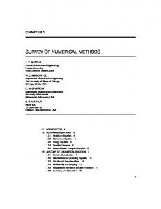
FIGURE 1. log2 (n) vs. CN T /n2

In addition to the above, we give a graph of n versus the actual counts of the integrand evaluations of K and Ku . The horizontal scale is log2 (n), and the vertical scale is the actual function count (CNT) divided by n2 . According to P1 and P2, these graphs should approach the values of 10/3 and 4/3 for K and Ku , respectively. These asymptotic limits are shown as horizontal lines in the graph; and indeed, the function counts approach these limits. This example is very typical of all of our examples to date. The program also shows that it is possible to solve quite inexpensively the large scale nonlinear systems associated with nonlinear integral equations. Two-grid vs. multigrid iteration. In the case of multigrid iteration, the rate of convergence increases as n increases, as stated in (4.17). But with either method, we need to compute only two iterates. (Actually one iterate is sufficient, but we prefer to be cautious


43

in checking for convergence in the iteration.) Thus the faster rate of convergence of the multigrid method is not needed in practice, as it produces an additional accuracy in the iterate that is not needed. Moreover, the multigrid method is more complicated to implement, and it costs somewhat more per iteration. An advantage of the multigrid method is that for larger values of n, it is generally safer to compute (1) only the one iterate xn for each n; whereas this is riskier with the twogrid iteration. Even with such a modification to the multigrid method, [4] found empirically that the multigrid method is still slower than the two-grid method in actual running time. For these reasons, we believe the two-grid iteration is to be preferred when solving integral equations. This discussion has been based on the use of composite numerical integration methods. However, in the linear case the best program resulted from using Gaussian quadrature; see IEGAUS in [10]. The performance of this latter program was much better than that of IESIMP or of any other standard composite rule; and thus we should also use Gaussian quadrature in place of Simpson’s rule in the construction of an automatic program for solving nonlinear integral equations. It should be noted that there is no known multigrid variant in this case. REFERENCES 1. E. Allgower, K. B¨ ohmer, F. Potra, and W. Rheinboldt, A mesh independence principle for operator equations and their discretizations, SIAM J. Num. Anal. 23 (1986), 160 169. 2. H. Amann, Zum Galerkin-Verfahren f¨ ur die Hammersteinsche Gleichung, Arch. Rational Mech. Anal. 35 (1969), 114 121. ¨ , Uber die Konvergenzgeschwindigkeit des Galerkin-Verfahren f¨ ur die 3. Hammersteinsche Gleichung, Arch. Rational Mech. Anal. 37 (1970), 143 153. 4. P. Anselone, ed., Nonlinear integral equations, University of Wisconsin, Madison, 1964. 5. , Collectively compact operator approximation theory and applications to integral equations, Prentice-Hall, New Jersey, 1971. 6. P. Anselone and R. Ansorge, Compactness principles in nonlinear operator approximation theory, Numer. Funct. Anal. Optim. 6 (1979), 589 618. 7. K. Atkinson, The numerical evaluation of fixed points for completely continuous operators, SIAM J. Num. Anal. 10 (1973), 799 807. 8. , Iterative variants of the Nystr¨ om method for the numerical solution of integral equations, Numer. Math. 22 (1973), 17 31.

44

K.E. ATKINSON

9. , A survey of numerical methods for Fredholm integral equations of the second kind, SIAM, Philadelphia, 1976. 10. , An automatic program for linear Fredholm integral equations of the second kind, ACM Trans. Math. Soft. 2 (1976), 154 171. 11. K. Atkinson and A. Bogomolny, The discrete Galerkin method for integral equations, Math. Comp. 48 (1987), 595 616. 12. K. Atkinson and G. Chandler, BIE methods for solving Laplace’s equation with nonlinear boundary conditions: The smooth boundary case, Math. Comp. 55 (1990), 451 472. 13. K. Atkinson and J. Flores, The discrete collocation method for nonlinear integral equations, submitted for publication. 14. K. Atkinson, I. Graham, and I. Sloan, Piecewise continuous collocation for integral equations, SIAM J. Num. Anal. 20, 172 186. 15. K. Atkinson and F. Potra, Projection and iterated projection methods for nonlinear integral equations, SIAM J. Num. Anal. 24, 1352 1373. 16. , The discrete Galerkin method for nonlinear integral equations, J. Integral Equations 1, 17 54. 17. C. Baker, The numerical treatment of integral equations, Oxford University Press, Oxford (1977), 685 754. ¨ 18. H. Brakhage, Uber die numerische Behandlung von Integralgleichungen nach der Quadraturformelmethode, Numer. Math. 2 (1960), 183 196. 19. F. Browder, Nonlinear functional analysis and nonlinear integral equations of Hammerstein and Urysohn type, in Contributions to nonlinear functional analysis (E. Zarantonello, ed.), Academic Press (1971), 425 500. 20. H. Brunner and P. van der Houwen, The numerical solution of Volterra equations, North-Holland, Amsterdam, 1986. 21. J. Flores, Iteration methods for solving integral equations of the second kind, Ph.D. thesis, University of Iowa, Iowa City, Iowa, 1990. 22. M. Ganesh and M. Joshi, Discrete numerical solvability of Hammerstein integral equations of mixed type, J. Integral Equations 2 (1989), 107 124. 23. , Numerical solvability of Hammerstein integral equations of mixed type, IMA J. Numerical Anal. 11 (1991), 21 31. 24. M. Golberg, Perturbed projection methods for various classes of operator and integral equations, in Numerical solution of integral equations (M. Golberg, ed.), Plenum Press, New York, 1990. 25. A. Griewank, The local convergence of Broyden-like methods on Lipschitzian problems in Hilbert space, SIAM J. Num. Anal. 24 (1987), 684 705. 26. W. Hackbusch, Multi-grid methods and applications, Springer-Verlag, Berlin, 1985. 27. G. Hsiao and J. Saranen, Boundary element solution of the heat conduction problem with a nonlinear boundary condition, to appear. 28. O. H¨ ubner, The Newton method for solving the Theodorsen integral equation, J. Comp. Appl. Math. 14 (1986), 19 30.


45

29. S. Joe, Discrete collocation methods for second kind Fredholm integral equations, SIAM J. Num. Anal. 22 (1985), 1167 1177. 30. H. Kaneko, R. Noren, and Y. Xu, Numerical solutions for weakly singular Hammerstein equations and their superconvergence, submitted for publication. 31. L. Kantorovich and G. Akilov, Functional analysis in normed spaces, Pergamon Press, London, 1964. 32. C.T. Kelley, Approximation of solutions of some quadratic integral equations in transport theory, J. Integral Equations 4 (1982), 221 237. , Operator prolongation methods for nonlinear equations, AMS Lect. 33. Appl. Math., to appear. 34. , A fast two-grid method for matrix H-equations, Trans. Theory Stat. Physics 18 (1989), 185 204. 35. C.T. Kelley and J. Northrup, A pointwise quasi-Newton method for integral equations, SIAM J. Num. Anal. 25 (1988), 1138 1155. 36. C.T. Kelley and E. Sachs, Broyden’s method for approximate solution of nonlinear integral equations, J. Integral Equations 9 (1985), 25 43. 37. , Fast algorithms for compact fixed point problems with inexact function evaluations, submitted for publication. 38. , Mesh independence of Newton-like methods for infinite dimensional problems, submitted for publication. 39. H. Keller, Lectures on numerical methods in bifurcation problems, Tata Institute of Fundamental Research, Narosa Publishing House, New Delhi, 1987. 40. J. Keller and S. Antman, eds., Bifurcation theory and nonlinear eigenvalue problems, Benjamin Press, New York, 1969. 41. M. Krasnoselskii, Topological methods in the theory of nonlinear integral equations, Macmillan, New York, 1964. 42. M. Krasnoselskii, G. Vainikko, P. Zabreiko, Y. Rutitskii, and V. Stetsenko, Approximate solution of operator equations, P. Noordhoff, Groningen, 1972. 43. M. Krasnoselskii and P. Zabreiko, Geometrical methods of nonlinear analysis, Springer-Verlag, Berlin, 1984. 44. S. Kumar, Superconvergence of a collocation-type method for Hammerstein equations, IMA J. Numerical Anal. 7 (1987), 313 326. 45. , A discrete collocation-type method for Hammerstein equations, SIAM J. Num. Anal. 25 (1988), 328 341. 46. S. Kumar and I. Sloan, A new collocation-type method for Hammerstein integral equations, Math. Comp. 48 (1987), 585 593. 47. H. Lee, Multigrid methods for the numerical solution of integral equations, Ph.D. thesis, University of Iowa, Iowa City, Iowa, 1991. 48. P. Linz, Analytical and numerical methods for Volterra integral equations, SIAM, Philadelphia, PA, 1985. 49. L. Milne-Thomson, Theoretical hydrodynamics, 5th ed., Macmillan, New York, 1968. 50. R.H. Moore, Newton’s method and variations, in Nonlinear integral equations, (P.M. Anselone, ed.) University of Wisconsin Press, Madison, WI, 1964.

46

K.E. ATKINSON

51. , Differentiability and convergence for compact nonlinear operators, J. Math. Anal. Appl. 16 (1966), 65 72. 52. , Approximations to nonlinear operator equations and Newton’s method, Numer. Math. 12 (1966), 23 34. 53. I. Moret and P. Omari, A quasi-Newton method for solving fixed point problems in Hilbert spaces, J. Comp. Appl. Math. 20 (1987), 333 340. 54. , A projective Newton method for semilinear operator equations in Banach spaces, Tech. Rep. #184, Dept. of Math., University of Trieste, Trieste, Italy, 1989. 55. W. Petryshyn, On nonlinear P -compact operators in Banach space with applications to constructive fixed-point theorems, J. Math. Anal. Appl. 15 (1966), 228 242. , Projection methods in nonlinear numerical functional analysis, J. 56. Math. Mech. 17 (1967), 353 372. , On the approximation solvability of nonlinear equations, Math. Ann. 57. 177 (1968), 156 164. 58. L. Rall, Computational solution of nonlinear operator equations, Wiley, New York, 1969. 59. K. Ruotsalainen and J. Saranen, On the collocation method for a nonlinear boundary integral equation, J. Comp. App. Math., to appear. 60. K. Ruotsalainen and W. Wendland, On the boundary element method for some nonlinear boundary value problems, Numer. Math. 53 (1988), 299 314. 61. J. Saranen, Projection methods for a class of Hammerstein equations, SIAM J. Num. Anal., to appear. 62. I. Sloan, Improvement by iteration for compact operator equations, Math. Comp. 30 (1976), 758 764. 63. D. Stibbs and R. Weir, On the H-function for isotropic scattering, Mon. Not. R. Astro. Soc. 119 (1959), 512 525. 64. G. Vainikko, Funktionalanalysis der Diskretisierungsmethoden, Teubner, Leipzig, 1976. 65. G. Vainikko and O. Karma, The convergence of approximate methods for solving linear and non-linear operator equations, Zh. v¯ y chisl. Mat. mat. Fiz. 14 (1974), 828 837. 66. R. Weiss, On the approximation of fixed points of nonlinear compact operators, SIAM J. Num. Anal. 11 (1974), 550 553. 67. E. Zeidler, Nonlinear functional analysis and its applications, Vol. I: Fixedpoint theorems, Springer-Verlag, Berlin, 1986.

Department of Mathematics, University of Iowa, Iowa City, IA 52242