A Survey of Recent Developments in DV-Hop Localization Techniques ...

A Survey of Recent Developments in DV-Hop Localization Techniques for Wireless Sensor Network Amanpreet Kaur1, Govind P Gupta2 and Padam Kumar1 1

Department of Computer Science & Engineering, Jaypee Institute of Information Technology, Noida, India. 2 Department of Information Technology, National Institute of Technology, Raipur, India. [email protected]

Abstract—In wireless sensor networks, localization is a required fundamental service to know the position of a sensor node within the network. The task of localization is performed after random deployment of all sensor nodes and is very useful in different types of services such as data tagging, node tracking, and target detection. Recently, numerous localization techniques based on DV-hop mechanism have been proposed. In this paper, we present a comprehensive survey of DV-hop localization techniques and make comparison of their approaches and performances. Based on the findings and analysis, some open research issues related to DV-hop localization techniques are suggested. Index Terms—Localization; DV-Hop; Wireless Sensor Network; Anchor; Localization Error; Energy Consumption.

I. INTRODUCTION A wireless sensor network (WSN) is a cooperative distributed system which consists of thousands small and resource-constrained sensor nodes and one or more sink node/nodes [1]. The main task of a sensor node is to observe physical phenomena and to transmit the observed data to the sink node through multi-hop communication [1-2]. In many applications of WSN such as environmental monitoring, battlefield surveillance, target tracking, position-based routing, medical care of old people, parking space detection, etc, geographical location of sensor nodes is required to detect the location of an event [1-4]. In the literature, localization techniques have been widely addressed since it is used for different types of locationbased services such as tracking of the sensor nodes, target detection, data tagging, clustering, topology control etc. The event information is not worthy if the location of node that has detected the given event is unknown. For example, in fire surveillance system, the location where fire (event) has occurred is as important as the detection of fire. Furthermore, the position of sensor nodes can be used in the optimization of different data routing and MAC protocols in WSN. A simple way to determine a node’s location is to equip a GPS on the sensor. However, the main limitation of GPS-based localization is that it does not work well in an indoor environment as well as dense areas such as forests and mountains, where GPS device may not get line-of-sight with GPS satellites. In addition, GPS device is very expensive and consumes a lot of energy for energyconstrained sensor node. WSN localization problem has drawn a huge attention from researchers and many solutions are proposed on this

research topic. In [3], Han et al. surveyed several localization schemes and classified them into different categories of range-based, range-free, historical information based, geometric based and time-based localization algorithms. Among all, range-free based localization schemes are very popular due to their low-cost service. The schemes use connectivity information between unknown nodes and anchor nodes for estimation of the node’s location. DV-hop based localization technique is recognized as the most popular technique and various variants of the improved DV-hop based localization schemes have been proposed in the literature [4-12]. In this paper, we present a comprehensive survey of the well-known DV-hop based localization techniques. This survey is different from the previous localization survey papers, as it includes almost all recent developments in the DV-hop based localization schemes since the beginning of 2013. The reason why the DV-Hop algorithm is chosen is that this is the most popular among all other localization algorithms because of its simplicity, cost effectiveness, scalability and accuracy. It is also suitable to find the location of even those nodes, which have less than three neighboring nodes. We discuss traditional DV-hop based localization algorithm, followed by a discussion on the different improvements suggested on the traditional DV-hop based schemes. Following the summary of the different improved DV-hop based schemes, we summarize the different DV-hop schemes in a table and discuss the performance analysis of these schemes in terms of communication overhead, accuracy and energy consumption. The rest of this paper is organized as follows. In Section II, we present related work most relevant to this paper. In Section II, we present traditional DV-hop based localization algorithm in details with its working example. Section III presents the state-of-the-art improved-DV-hop based localization algorithm. In Section IV, we discuss the performance analysis of all variants of DV-Hop based on their working approach and performance metrics. Finally, we conclude the paper with some future research issues. II. TRADITIONAL DV-HOP ALGORITHM This section presents the description of traditional DVHop localization algorithm and its limitations. The parameters and variables used in the description of the DVHop algorithm are described in Table 1.

ISSN: 2180-1843 e-ISSN: 2289-8131 Vol. 9 No. 2

61

Journal of Telecommunication, Electronic and Computer Engineering

Niculesco and Nath [4] proposed one of the best-known range-free approach based localization algorithm, called DV-Hop algorithm. It is a distributed hop-by-hop localization scheme that gives an approximate location of all nodes in a network by using a small number of GPSequipped sensor nodes. In this algorithm, each node first calculates its minimum hop count to the anchor node and then estimates the distance between the node and the anchor node. Each node estimates its location using triangulation mechanism. The pseudo code of DV-Hop Algorithm is depicted in Algorithm 1.

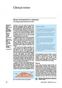
count from each anchor. In this example, Node N is 3 hop counts away from anchor A1, 3 hop counts away from anchor 2 and 2 hop counts away from anchor A3. The Anchor A1 is 3 hop counts far from anchor A2 and is at the distance of 5 hop counts from anchor A3. The Anchor A2 is 5 hop counts far from A3.

Table 1 Symbol Table for DV-Hop Algorithm Symbol i (xi,yi) hi Ahdi

Description ID for a node. x and y coordinates of node Hop count from anchor i. Average distance per hop computed by anchor i Figure 1: Example of DV-Hop localization algorithm

Algorithm 1: Pseudo Code of DV-Hop Algorithm 1. For each anchor i, (a) Set hopcount hi =0. (b) Broadcast self location (i, xi,yi,hi) to all neighbours. 2. For each receiving neighbour, (a) Let hir=hi received in the packet, and hit=hopcount stored in its hopcount table (b) If hit=0 or hir < hit-1,then hir=hir+1 Set hit=hir broadcast the packet(i, xi,yi,hir) to all neighbours. else discard packet 3. For each anchor i, (a) Compute Ahdi. (b) Broadcast Ahdi to all neighbours 4. For each receiving node, (a) Compute distance from every anchor. (b) Compute its location using least square method. 5. Stop

DV-hop algorithm works in three phases that are described as follows: Phase 1: Determining minimum hop counts of every node: In this phase, each anchor node conveys its location information to its neighbor nodes, which further conveys to its neighbor nodes so that all the nodes in the network get this information by broadcasting a small packet. The packet contains information where xi,yi are x and ycoordinates of anchor i and hi represents hop count. The initial value of hi is 0. Each node maintains its hop count table containing for each anchor i. When the packet is received by any node, it checks its own table and if the value of hi stored in its table is less than hi value received by it, then it ignores that received value; otherwise it increments hi value by 1 and stores the new value of hi for anchor i in its table. After saving this value, it forwards the packet with updated value of hi to all its neighbors. In this way, after the first phase, each node gets minimum hopcount from every anchor node and has updated hop-count table. Figure 1 illustrates the working of Phase 1. In Figure 1, there are three anchors A1, A2, A3 and unknown node N in a wireless sensor network. All these three anchors convey their message containing information about their location and hop count to all other nodes in the network. All the nodes after receiving the given message, update their hop count table. For example, after phase 1, unknown node N has updated the hop count table as shown in Table 2. The unknown node N gets the minimum hop 62

Table 2 Table containing for each anchor i maintained by node N Anchor id 1 2 3

xi coordinate 100 250 400

yi coordinate 200 400 100

Hop counts 3 3 2

Phase 2: Determining average hop distance: In this phase, each anchor Ai estimates average distance per hop(AvgHopDistancei) using Equation (1). AvgHopDistancei =

2 2 ∑n j=1 j#i √(xi −xj ) + (yi − yj )

∑n j=1 j#i hj

(1)

where n is the total number of anchors in the network, j denotes all other anchors and hj is the number of hops between anchor i and anchor j, (xi,yi) and (xj,yj) represents coordinates of anchors i and j, respectively. After computing average hop distance, each anchor Ai broadcasts it in the network. Then, each node i who does not know its location computes its distance from the anchor Ai using Equation (2). 𝑑𝑖 = 𝐴𝑣𝑔𝐻𝑜𝑝𝐷𝑖𝑠𝑡𝑎𝑛𝑐𝑒𝑖 × ℎ𝑖

(2)

For the network, as shown in Figure 1, anchor A1, A2 and A3 first compute their average hop distances using Equation (1). Thus, anchor A1, A2 and A3 determine their average hop distances from each anchor using Equation (1), as shown in Table 3. The anchor A1 computes its average hop distance as shown below: 𝐴𝑣𝑔𝐻𝑜𝑝𝐷𝑖𝑠𝑡𝑎𝑛𝑐𝑒1 =

√(𝑥1 −𝑥2 )2 +(𝑦1 −𝑦2 )2 +√(𝑥1 −𝑥3 )2 +(𝑦1 −𝑦3 )2 ℎ2 +ℎ3

that is, 𝐴𝑣𝑔𝐻𝑜𝑝𝐷𝑖𝑠𝑡𝑎𝑛𝑐𝑒1 =

√(100−250)2 +(200−400)2 +√(100−400)2 +(200−100)2 3+5

= 70.7

Similarly, in this way, anchors A2 and A3 computes its average hop distances.

ISSN: 2180-1843 e-ISSN: 2289-8131 Vol. 9 No. 2

A Survey of Recent Developments in DV-Hop Localization Techniques for Wireless Sensor Network Table 3 Average Hop distances computed by each anchor i in phase 2 Anchor i A1 A2 A3

Equation (5) can be re-written as follows: X = (AT A)−1 AT B

AvgHopDistancei 70.7 73.2 65.2

The unknown node N determines its distance from each anchor Ai using Equation (2), and the distances computed by node N is shown in Table 4. Thus, the node N, which is 3 hop counts away from anchor A1 determines its distance from anchor A1 as follows: 𝑑1 = ℎ3 × 𝐴𝑣𝑔𝐻𝑜𝑝𝐷𝑖𝑠𝑡𝑎𝑛𝑐𝑒1 𝑑1 = 3 × 70.7 =212.20

that is,

In the similar way, the node N determines its distances from other anchors A2 and A3. Table 4 Distance computed by node N from every anchor i in phase 2 Anchor i A1 A2 A3

Distance(di) 212.1 219.6 130.4

Phase 3: Determining coordinates of an unknown node using multilateration: In this phase, each unknown node uses multilateration method to determine its location. The information, that is the unknown node required for this phase is the coordinates of all anchor nodes and their distance from each anchor obtained from phase 2 of DV-hop localization algorithm. The multilateration method works as follows: Let (xn,yn) be the coordinates of unknown node N and (xi,yi) be the coordinates for anchor Ai and let there are total m anchors. Then, we can get the following system of equations: (xn − x1 )2 + (yn − y1 )2 = d1 2 (xn − x2 )2 + (yn − y2 )2 = d2 2 ⃛⋮ (xn − xm )2 + (yn − ym )2 = dm 2

(3)

Subtracting all equations one by one by the last equation in (3), we get the following Equation (4): 2 2 x12 − xm + y12 − ym − d12 − d2m = 2 × xn × (x1 − xm ) + 2 × yn × (y1 − yn ) 2 2 x22 − xm + y22 − ym − d22 − d2m = 2 × xn × (x2 − xm ) + 2 × yn × (y2 − yn ) ⋮ 2 2 2 2 xm−1 − xm + ym−1 − ym − d2m−1 − d2m = 2 × xn × (xm−1 − xm ) + 2 × yn × (y1 − yn )

(4)

Equation (4) can be written in the form of matrix equation as follows:

where:

and

x1 − xm x2 − xm A =2×[ ⋮ xm−1 − xm

B=

x12 x22

− −

2 xm 2 xm

+ +

y12 y22

The coordinates of the nodes are determined by solving Equation (6) using the Least square method [4]. The advantage of DV-Hop Algorithm is that this algorithm is cost effective and can be used to find the location of all nodes even if the node has less than three neighboring anchors as compared to the other range-free algorithms. It is also much more accurate. The disadvantage of this algorithm is that it can only be used for isotropic networks and its accuracy still needs to be considered when compared with the range-based algorithms as it gives the approximate location. Despite the fact that DV-Hop [4] has many points of interest, there is still much scope for improvement in terms of localization accuracy. Since the localization accuracy is affected by the number of anchor nodes and its position in the network, the distance between the normal nodes and the anchor nodes. Thus, many improvements are suggested in the recent years in the literature [5-12]. In the following section, several improved versions of the traditional DVHop localization algorithms will be further described. III. IMPROVED VERSIONS OF THE TRADITIONAL DV-HOP ALGORITHM In this section, we discuss 13 improved versions of the traditional DV-Hop localization algorithms proposed in the recent years to estimate the location of unknown nodes in WSNs. The first phase in all the algorithms is similar to the phase 1 of DV Hop Algorithm. Thus, we skip Phase 1 in all the improved algorithms. The output of the first phase is that all the unknown nodes get minimum hop counts hi from every anchor i. A. An Improved DV-Hop Localization Algorithm (IDVLA) In [5], H.Chen et al. proposed a fast, accurate and easy-touse DV-Hop Localization Algorithm (IDVLA), which improves accuracy as well as coverage. The working of this algorithm consists of three phases. Phase 2: Refinement of phase 2 of Traditional DV-Hop Algorithm: This phase is used to determine average hop distance by each anchor. Each anchor uses Equation (1) to compute its average hop distance and broadcasts it to every other node. The unknown node whose location needs to be found maintains a table containing average hop distances from each anchor i. Then it computes the average of these entire average hop distances to get the average hop distance using Equation (7). 𝐻𝑜𝑝𝑆𝑖𝑧𝑒𝑎𝑣 =

(5)

AXn=B y1 − ym y2 − y m xn ], Xn = [y ], ⋮ n ym−1 − ym 2 ym 2 ym

d12 d22

d2m d2m

− − − − − − ⋮ 2 2 2 2 [xm−1 − xm + ym−1 − ym − d2m−1 − d2m ]

(6)

∑ 𝐴𝑣𝑔𝐻𝑜𝑝𝐷𝑖𝑠𝑡𝑎𝑛𝑐𝑒𝑖 𝑛

(7)

Then, each unknown node computes its distance from each anchor I, using Equation (8). 𝑑𝑖 = ℎ𝑖 × 𝐻𝑜𝑝𝑆𝑖𝑧𝑒𝑎𝑣

(8)

Phase 3: Improved phase for determining the location of unknown node: In this phase, each unknown node determines its location using 2-D Hyperbolic [5] location

ISSN: 2180-1843 e-ISSN: 2289-8131 Vol. 9 No. 2

63

Journal of Telecommunication, Electronic and Computer Engineering

algorithm instead of the least square method. This method takes new distances computed in the second phase to find the location. The whole process is explained in detail in [5]. It is observed that if anchors are deployed uniformly, then the performance of IDVLA algorithm increases. Experimental results show that with 10% anchor nodes, the IDVLA algorithm reaches improved location coverage about 100% and accuracy is improved by 9% with 5% anchor nodes [5]. Thus, IDVLA algorithm improves accuracy and coverage as compared to traditional DV-Hop Algorithm. B. Weighted Centroid Localization Algorithm (WCL) The Weighted Centroid Localization Algorithm (WCL) was proposed in [6] to improve computational complexity of DV-hop localization scheme. WCL contains two phases. Phase 2: Determining the location of unknown node: After completion of the first phase, in the second phase, every unknown node computes its location (xu, yu) using Equation (9). 𝑥𝑢 = where 𝑤𝑖 =

1 ℎ𝑖

∑𝒏 𝒊=𝟏 𝒘𝒊 𝒙𝒊 ∑𝒏 𝒊=𝟏 𝒘𝒊

, 𝑦𝑢 =

∑𝒏 𝒊=𝟏 𝒘𝒊 𝒚𝒊 ∑𝒏 𝒊=𝟏 𝒘𝒊

(9)

, is the weight of each anchor i.

Experimental results show that the performance of WCL algorithm is almost the same as that of DV-Hop [4] algorithm in terms of accuracy. However, the computational complexity of WCL algorithm is less than the DV-Hop algorithm, as it contains one less phase than the DV-Hop algorithm. C.

An Improved Weighted Centroid Algorithm based on DV-Hop In [6], B.Zhang et al. proposed another improved weighted centroid algorithm based on DV-Hop (IWCL) to improve accuracy. The IWCL algorithm consists of two phases. Phase 1: Determining the minimum hop counts of every node: In this phase, all unknown nodes try to determine a minimum number of hops from every anchor and maintain the hop count table. Then, they sort these hop counts with each anchor node in ascending order and select a few anchor nodes whose hop count is quite small. Phase 2: Determining the location of unknown node: In this phase, each anchor computes its average hop distance using Equation (1) and sends this to the unknown node. The unknown node determines the average of all these averages of hop distances using Equation (7). The unknown node then computes their location using Equation (9). The weight used in Equation (9) is computed using Equation (10).

selected to compute the location of an unknown node is not mentioned in phase 1. D. An Improved DV-Hop Localization (IDV-Hop) In [7], W.Yu et al proposed an improved DV-Hop (IDVHop) localization algorithm which adds a correction step while computing the distance between an unknown node and anchor in the second phase in order to improve accuracy. This algorithm works in three phases: Phase 2: Determining the distance between an unknown node and an anchor: In this phase, firstly, every anchor i computes its average hop distance using Equation (1). Till now, the steps are the same as that of the original DV-Hop Algorithm. Now, a refinement is done to improve the performance of the algorithm. The correction is calculated by the unknown node N, using Equation (11). 𝑐𝑖 =

𝐻𝑜𝑝𝑆𝑖𝑧𝑒

(10)

𝑎𝑣 where 𝑛 = ( ) and r is the communication radius of 𝑟 the node. The simulation results show that IWCL algorithm performs better than DV-Hop Algorithm in terms of accuracy. The advantage of IWCL algorithm is that it is more accurate and less complex as it has only two phases. The drawback is that the number of anchors needs to be

64

𝑟

(11)

where ci is the correction, hi is the minimum hop counts of anchor i from node N, r is the communication radius and AvgHopDistancei is the average Hop Distance computed by anchor i using Equation (1). Then, the distance between the unknown node N and anchor i is computed using Equation (12). 𝑑𝑖 = (ℎ𝑖 × 𝐴𝑣𝑔𝐻𝑜𝑝𝐷𝑖𝑠𝑡𝑎𝑛𝑐𝑒𝑖 ) + 𝑐𝑖

(12)

Phase 3: Determining the location of unknown node: The third phase is the same as that of the original DV-Hop algorithm [4]. As in this algorithm, one correction step is added, thus it increases computational complexity of the given algorithm to some extent, though the accuracy is improved over the original DV-Hop Algorithm. The simulation results show that the accuracy is improved by 1.5% to 4% than the original DV-Hop algorithm by varying anchor nodes. E. Hybrid DV-Hop Algorithm (HDV-Hop) H.Safa et al. [8] proposed Hybrid DV-Hop (HDV-Hop) localization algorithm to minimize localization error, flooding and power consumption. In this algorithm, the authors assumed that anchors are deployed on the perimeter of the network. The HDV-Hop algorithm works in four phases. The symbol table used for this algorithm is described in Table 5: Table 5 Symbol Table for HDV-Hop Algorithm Symbol min(hi) Gmn

1

1 𝑛 ℎ𝑖

𝑤𝑖 = ( )

(ℎ𝑖 ×(𝑟− 𝐴𝑣𝑔𝐻𝑜𝑝𝐷𝑖𝑠𝑡𝑎𝑛𝑐𝑒𝑖 )

Pa HopCount Table

Description Minimum hop value from anchor i for given node. Global minimum neighbor. It is a node which is at distance of one hop from the given node and has sent min(hi) Parent anchor. It is an anchor for which min(hi) value corresponds. Table maintained by all nodes containing values for every anchor i

Phase 1: Determining minimum hop counts, global minimum neighbor and parent anchor by every node: In this phase, as in the original DV- Hop [4], the anchors send their location and hi value to all other nodes in the network. The unknown nodes maintain a Hop count table having values for every anchor i. Unlike the first phase of the

ISSN: 2180-1843 e-ISSN: 2289-8131 Vol. 9 No. 2

A Survey of Recent Developments in DV-Hop Localization Techniques for Wireless Sensor Network

traditional DV-Hop Algorithm, each unknown node also keeps a record of where min (hi) is the minimum hop value from anchor i in its table, gmn (global minimum neighbor) is one hop neighbor of that node, which has sent this min(hi) value, and pa (parent anchor) is the anchor i for which this min(hi) value corresponds. Only these gmn and pa nodes will be used for communication with the base station by the given node. Phase 2: Determining average hop length by each anchor: In this phase, each anchor computes its average hop distance using Equation (1) and sends it to the base station using only anchors. The base station is assumed to be deployed on the perimeter of the network and can only communicate with anchors. In traditional DV-Hop Algorithm, each anchor sends its average hop distance to every node in the network, but in HDV-Hop algorithm, this message of average hop distance by the anchor is sent only to base station using nodes and anchors which come in between node and base station. This change is made to reduce flooding and power consumption as now less number of nodes and anchors are involved in this communication. When the unknown sensor node detects an event, the node needs to report this event to the base station. The unknown node sends the sensed data and its Hop Count table in the form of a packet to its gmn, which in turn sends it to its gmn till it reaches its pa. Then the pa of unknown node forwards this packet to the base station using all the anchors which come in between pa and base station. The routing protocol is required for this phase to find the shortest path from the reporting sensor node to the base station. This phase is absent in the traditional DV-Hop algorithm [4]. No routing protocol is required for traditional DV-Hop algorithm also. Phase 3: Computing location of unknown reporting sensor node by base station: To get the location of the reporting sensor node, the base station utilizes the information containing Hop count table sent by the node in the form of a packet and computes the distance of a given node from each anchor, using Equation (2). After computing all the distances of the unknown node from all the anchors, the base station uses trilateration method to get the location of the given node. Unlike traditional DV-Hop algorithm, which uses linear LS technique [4] for multilateration phase, this non-linear technique uses the Levenberg-Marquardt (LM) algorithm [8] . The LM technique is used as it gives the best results in terms of accuracy and is best suitable for non-linear equations when compared with other optimization techniques in [8]. The advantage of HDV-Hop algorithm is that it reduces flooding. The anchors and the unknown node must send the message to the nodes and anchors, which are connected with the base station. Most of the computation is now done by the base station. The simulation and results in [8] show that this algorithm reduces location error and power consumption when compared with the original DV-Hop algorithm [4]. The drawback of this algorithm is that anchors and base station in this algorithm needs to be deployed outside the network. If base station fails, then this algorithm will not work. The routing protocol is required to get the shortest path from the unknown node to parent anchor and to get the path from anchor to the base station.

F. An improved localization algorithm based on genetic algorithm (GADV-Hop) Bo.Peng et al [9] proposed an improved DV-Hop localization algorithm based on genetic algorithm, called GADV-Hop algorithm. GADV-Hop uses the genetic algorithm to improve the accuracy of Traditional DV-Hop algorithm [4]. It consists of three phases. The working of GADV-Hop algorithm is as follows: Phase 2: Determining the distance between unknown nodes with every anchor: The second phase is similar to the second phase of Traditional DV-Hop Algorithm [4]. First, each anchor determines its average hop distance using Equation (1) and then secondly, each unknown node computes its distance from each anchor using Equation (2). Phase 3: Applying genetic Algorithm on each unknown node: In the third phase, the genetic algorithm is applied to improve the accuracy of localization algorithm. The genetic algorithm is discussed in detail in [9]. The advantage of this algorithm is that this algorithm performs better than the Original DV-Hop algorithm as it results in lower localization error and is much more stable. However, the disadvantage of this algorithm is that it increases its computational complexity due to the genetic algorithm. It is observed that if the genetic algorithm is applied to original DV-Hop, then accuracy improves. G. Hyperbolic DV-Hop Localization algorithm In [10], G.Song et al. proposed the Hyperbolic DV-Hop algorithm used to improve accuracy which refines the second and third phase of the traditional DV-Hop algorithm. The working of this algorithm is divided into three phases: Phase 2: Determining the distance between unknown nodes with every anchor: Unlike the second phase of the Traditional DV-Hop algorithm, where each anchor computes its average hop distance using Equation (2), here in this phase, the unknown node computes the average of all average hop distances of all anchor nodes using Equation (13). 𝐴𝑣𝑒𝑟𝑎𝑔𝑒𝐻𝑜𝑝𝑑𝑖𝑠𝑡𝑎𝑛𝑐𝑒 =

∑𝑚 𝑖=1 𝐴𝑣𝑔𝐻𝑜𝑝𝐷𝑖𝑠𝑡𝑎𝑛𝑐𝑒𝑖 𝑚

(13)

where m is the total number of anchors and AvgHopDistancei is the average hop distance computed by each anchor i using Equation (2). Then, the unknown node computes its distance from each anchor i using Equation (14). 𝑑𝑖 = 𝐴𝑣𝑔𝐻𝑜𝑝𝐷𝑖𝑠𝑡𝑎𝑛𝑐𝑒 × ℎ𝑖

(14)

This refinement is done to reduce the error in computing average hop distance as now all the anchors are considered instead of considering the nearest anchor only. Phase 3: Trilateration Phase: In this phase, Trilateration technique uses more accurate hyperbolic location algorithm to compute the location of an unknown node rather than using LS technique as in the Traditional DV-Hop algorithm. This hyperbolic location algorithm is explained in [10]. Compared to the original DV-Hop algorithm, Hyperbolic DV-Hop algorithm has improved the accuracy from 8 to 10%.

ISSN: 2180-1843 e-ISSN: 2289-8131 Vol. 9 No. 2

65

Journal of Telecommunication, Electronic and Computer Engineering

H. Improved Weighted Centroid DV-Hop Localization Algorithm (IWCDV-Hop) Hyperbolic-DV-Hop Algorithm improves accuracy to a small extent, thus in [10], G.Song et al. proposed a second localization algorithm called as the improved weighted centroid DV-Hop(IWCDV-Hop) localization algorithm. This algorithm makes use of a centroid concept to improve accuracy by a large extent. The IWCDV-Hop Algorithm works in two phases discussed as follows: Phase 2: Computing location of unknown node: The second phase of Original DV-hop is missing in it. In this algorithm, every unknown node computes its location (xu,yu) using Equation (15). 𝒙𝒖 =

∑𝒏 𝒊=𝟏 𝒘𝒊 𝒙𝒊

𝒚𝒖 =

∑𝒏 𝒊=𝟏 𝒘𝒊

∑𝒏 𝒊=𝟏 𝒘𝒊 𝒚𝒊 ∑𝒏 𝒊=𝟏 𝒘𝒊

(15)

where n is the total number of anchors in the network, and (xi,yi) are the coordinates of each anchor i, wi is the weight of anchor i , which is computed using Equation (16). 𝑤𝑖 =

∑𝑛 𝑖=1 ℎ𝑖

(16)

𝑛ℎ𝑖

This algorithm has a minimum number of steps as compared with all the previous DV-hop based localization algorithms. Thus, it reduces the computational complexity of the given algorithm. In other centroid based DV-Hop algorithms [20, 21], threshold variable is used whose value decides the number of anchors used for computing the location of the node. If the distance of anchor from the given node is less than the threshold value, then only that anchor is considered for trilateration phase. For this algorithm, threshold variable is not required. This algorithm uses all the anchor nodes in the network to compute the location of an unknown node which improves its accuracy. The choice of the threshold value is in itself a very complex problem. As this algorithm does not use threshold value, this step of finding threshold value is missing here. Compared to the original DV-Hop, IWCDV-Hop increases its accuracy from 59% to 63%. I. CheckOut DV-Hop Algorithm In [11], L.Gui et al. proposed CheckOut DV-Hop Localization algorithm in which one more phase called checkout phase is added to improve the accuracy. In this algorithm, the unknown node makes use of the nearest anchor to compute its location. The working of this algorithm is divided into four phases. The symbol table used in this algorithm is shown in Table 6. Table 6 Symbol Table for CheckOut DV-Hop Algorithm Symbol Ni (xi,yi) Anear ddv-hop dnear,i

Description An unknown node having ID i. Coordinates of unknown node obtained after the third phase Nearest anchor to given node having minimum number of hop counts from given node. Distance between unknown node Ni and Anear computed in the third phase. Distance between unknown node Ni and Anear computed using Equation (2).

Phase 2: Determining distance between unknown nodes with every anchor: This phase is the same as that of the

66

traditional one. In addition to this, each unknown node N i finds the nearest anchor Anear , which has a minimum number of hop counts from it. Let the distance of an unknown node from Anear be dnear,i using Equation(2). Phase 3: Determining coordinates of an unknown node using multilateration phase: This phase is the same as that of the third phase of the traditional one. Then, the location of unknown node i is computed using trilateration method. Let the coordinates of node i computed be . Then, each of the unknown nodes i find its distance from its nearest anchor Anear as ddv-hop. Phase 4: Checkout phase: One low-computational phase called Checkout phase is added in this algorithm. In this phase, the location of unknown node i is computed using Equation (17). ddv−hop − dnear,i 𝑥𝑐ℎ𝑒𝑐𝑘𝑜𝑢𝑡 = 𝑥𝑖 − ( ) ∗ (𝑥𝑖 − 𝑥𝑎𝑛𝑒𝑎𝑟 ) dddv−hop ddv−hop − dnear,i 𝑦𝑐ℎ𝑒𝑐𝑘𝑜𝑢𝑡 = 𝑌𝐼 − ( ) ∗ (𝑦𝑖 − 𝑦𝑎𝑛𝑒𝑎𝑟 ) ddv−hop

(17)

where (xanear,yanear) are the coordinates of anchor Anear. This fourth phase requires small computations, so it does not really affect computational complexity. The computational complexity is almost the same as that of the original DV-Hop algorithm. Checkout DV-Hop Localization algorithm improves the accuracy by 10 to 25% as compared to the original DV-Hop algorithm. J. Selective 3-Anchor DV-Hop Algorithm L.Gui et al. [11] proposed a selective 3-Anchor DV-Hop algorithm, which makes use of only 3 anchors to compute the coordinates of an unknown node. The working is divided into three phases. Phase 2: Determining distance between unknown nodes with every anchor: This phase is the same as that of the second phase of the traditional one. Phase 3: Determining coordinates of an unknown node using multilateration phase: The location of an unknown node is computed by using only 3 most accurate anchors instead of using all the anchors as in the traditional DV-Hop Algorithm. Experimental results show that the use of this algorithm improves accuracy by 18 to 30% in different scenarios as compared to the original DV-Hop algorithm. The computational complexity increases in this algorithm because of the third step which requires a very complex and time-consuming procedure to find three most suitable anchors. K. Improved DV-Hop 1 Algorithm (iDV-Hop1) In [12], S. Tomic et al. proposed an improved DV-Hop algorithm, called iDV-Hop1 algorithm to improve accuracy in all types of scenarios by using geometry. It consists of four phases: Phase 2: Determining distance between unknown nodes with every anchor: The second phase is also similar to the second phase of traditional DV-Hop algorithm. Phase 3: Determining coordinates of an unknown node using multilateration phase used in the original DV-Hop algorithm: The third phase is also similar to the third phase of the traditional DV-Hop algorithm. Let (xDV,yDV) be the nodes of unknown node N obtained after third phase of original DV-Hop algorithm and (xnear, ynear) be the anchor

ISSN: 2180-1843 e-ISSN: 2289-8131 Vol. 9 No. 2

A Survey of Recent Developments in DV-Hop Localization Techniques for Wireless Sensor Network

which is the nearest to the given node N having the minimum number of hops from node N. Phase 4: Determining coordinates of unknown node using geometry method: Two circles of radius Rnear and Rn computed using Equations (18) and (19) respectively, are drawn around anchor Anear and the unknown node N. 𝑅𝑛𝑒𝑎𝑟 = (𝑥𝐷𝑉 − 𝑥𝑛𝑒𝑎𝑟 )2 + (𝑦𝐷𝑉 − 𝑦𝑛𝑒𝑎𝑟 )2

(18)

𝑅𝑛 = 𝐴𝑣𝑔𝐻𝑜𝑝𝐷𝑖𝑠𝑡𝑎𝑛𝑐𝑒𝑛𝑒𝑎𝑟 × ℎ𝑛𝑒𝑎𝑟

(19)

where AvgHopDistancenear and hnear are average hop distance per hop computed by anchor Anear in the second phase and the minimum number of hops computed by node N from anchor Anear in the first phase. These two circles intersect at two points S1(xs1,ys1) and S2(xs2,ys2). Then, the coordinates of unknown node N (xiDV1,yiDV1) is calculated using centroid formula in Equation (20) as follows: xnear + xs1 + xs2 3 ynear + ys1 + ys2 = 3

xiDV1 = yiDV1

(20)

The simulation results show that iDV-Hop1 algorithm improves accuracy up to three times in scenarios with irregular topology as compared with original DV-Hop algorithm. However, the iDV-Hop1 algorithm has increased computational complexity as compared to original DV-Hop algorithm due to the addition of fourth phase containing geometry. L. Improved DV-Hop 2 Algorithm (iDV-Hop2): In [12], S.Tomic et al. proposed a second improved algorithm based on geometry to improve accuracy as compared with the original DV-Hop algorithm for all scenarios and with iDV-Hop1 for scenarios with regular topologies. It works in four phases: Phase 2: Determining distance between unknown nodes with every anchor: The second phase is also similar to the second phase of the traditional DV-Hop algorithm. Phase 3: Determining coordinates of an unknown node using multilateration phase used in the original DV-Hop algorithm: The third phase is also similar to the third phase of the traditional DV-Hop algorithm. Let (xDV,yDV) be the nodes of unknown node N obtained after the third phase of the original DV-Hop algorithm and (xnear, ynear) be the anchor which is the nearest to the given node N having the minimum number of hops from node N. Phase 4: Determining coordinates of an unknown node using geometry method: In the fourth phase, the unknown node N first forms two circles and finds two intersection points S1(xs1,ys1) and S2(xs2,ys2), which is the same as in the iDV-Hop1 Algorithm. Then, the coordinates of unknown node N (xiDV2,yiDV2) is calculated using the centroid formula in Equation (21) as follows: xDV + xs1 + xs2 3 yDV + ys1 + ys2 = 3

xiDV2 = yiDV2

(21)

The simulation results prove that the iDV-Hop 2 algorithm has up to 11 % lower localization algorithm than

the iDV-Hop 1 Algorithm and the original DV-Hop Algorithm. The computational complexity of iDV-Hop 1 is much more than the original DV-Hop algorithm because one more phase is using geometry method and it is almost the same when compared with the iDV-Hop 1 algorithm. M. Quadratic DV-Hop Algorithm (Quad DV-Hop algorithm): In [12], S.Tomic proposed the third algorithm called Quad DV-Hop algorithm to reduce localization error, in which a refinement in the third step of the original DV-Hop algorithm is made. The work of Quad DV-Hop algorithm is divided into three phases: Phase 2: Determining distance between unknown nodes with every anchor: The second phase is also similar to the second phase of the traditional DV-Hop algorithm. Phase 3: Determining coordinates of an unknown node using quadratic program (QP) method: The third phase is modified to improve accuracy in the Quad DV-Hop Algorithm. The least squares problem is first considered and converted into the quadratic program (QP), which is then, solved using quadratic programming solver. The whole process is explained in detail in [12]. Simulation results prove that the Quad DV-Hop algorithm gave better performance in all types of scenarios when compared with the original DV-Hop algorithm, but it has high computational complexity due to the use of QP solver. IV. DISCUSSION AND OPEN RESEARCH ISSUES We reviewed all variants of the DV-Hop localization algorithms proposed for WSNs in the previous sections. In this section, we summarize the main features of these localization algorithms, compare their performances and reveal some open research issues. A. Comparison of all variants of DV-Hop algorithms based on their approaches In this section, we present the comparison of different DV-hop based localization algorithms. First, we compare these algorithms based on their approaches adopted in the design of the different working phase of the localization protocol. Next, we present the performance comparison of these localization algorithms based on different performance metrics such as computation complexity, accuracy, and energy consumption. After an extensive review of all variants [4-12] of the DVHop based localization algorithms, we observed that the majority of these algorithms are distributed and adopted an estimation based mechanism for location estimation of the normal sensor nodes. Distributed algorithm is very useful for large-scale WSNs where generally online localization mechanism is more practical and convenient. Among the surveyed DV-Hop localization algorithms, it was observed that the first phase in all algorithms is the same as that of the original DV-Hop [4]. IDVLA Algorithm [5] refines its second phase by taking the average of the average hop distances computed by each anchor (refer Equation (7)) and its third phase by replacing the least square method with a more accurate 2-D Hyperbolic location method to improve the localization accuracy. Weighted Centroid method is used in WCL [6], IWCL [6] and IWCDV [10] and this method considers weight that depends on hop count, linked with each anchor to compute the location of an unknown node. In

ISSN: 2180-1843 e-ISSN: 2289-8131 Vol. 9 No. 2

67

Journal of Telecommunication, Electronic and Computer Engineering

IDV-Hop [7], correction value using Equation (11) is computed and added in the distance computed by an unknown node from each anchor to reduce localization error. This modified distance is then used in the third phase to compute the location of the node. Among all DV-Hop based schemes, HDV-Hop [8] uses centralized approach for computation of the coordinates of the unknown sensor nodes. GADV-Hop [9] algorithm uses a genetic algorithm to minimize the total estimation error of the localization problem. However, the computation complexity of the GADV-Hop algorithm is very high. Hence, there is a tradeoff between localization error and computation complexity for this scheme. In Hyperbolic-DV [10], the average hop-size of the unknown node is calculated as an average of the average hop-sizes of all the anchor nodes, instead of taking the average hop-size of anchor node closest to the unknown node. This approach improves the accuracy of the location estimation. Checkout DV-hop [11] algorithm has an additional fourth phase of Checkout-Algorithm where checkout is applied to get better localization accuracy. Selective 3-anchor DV-hop [11] algorithm uses only the three most accurate anchors to determine the coordinates of an unknown node in multilateration phase (third phase) instead of using all the anchors as in the original DV-Hop algorithm. This refined phase which requires the complex method to select three anchors among all anchors put an extra burden on the computational complexity on the algorithm. IDV-Hop1[12] and IDV-Hop2[12] Algorithms compute location using geometry methods and have one more phase than other algorithms. Quad-DV-Hop [12] Algorithm uses QP method in the third phase which improves accuracy but increases computational complexity. We observed that for most of the proposed variants of the DV- Hop localization, average localization error decreases as the number of the anchor nodes increases and also it increases as the communication range increases. B. Comparison of all variants of DV-Hop algorithms based on performance metrics In this section, we present the performance analysis of all variants of DV-hop based localization algorithms in terms of different evaluation metrics such as computation complexity, localization accuracy and energy consumption. Computation complexity/cost depends on the number of phases and number of steps in each phase. The more the number of steps or phases, the more is the computation cost of localization algorithm. Localization accuracy is the most important performance metric for comparison of the localization algorithms. Localization accuracy can be measured in terms of localization error [22]. The localization error is equal to the difference between absolute location and estimated location determined by the localization algorithm. Due to the limited energy budget at each sensor nodes, energy consumption is a very important metric used for comparison of the protocols design for WSNs. The main component responsible for energy consumption at a sensor node is due to the communication unit. The communication cost is determined by the total number of packets transmitted and received by each node. Thus, energy consumption can be reduced by reducing communication overhead between nodes. In Table 7, we summarized the comparison of all variants of DV-Hop

68

algorithms in terms of computation complexity, localization accuracy and energy consumption. Among all surveyed DV-Hop based localization algorithms, we observed that traditional DV-Hop [4] algorithm has low accuracy compared to all its variants. All other variants of DV-Hop have been proposed mainly to improve its localization accuracy. Due to flooding in the first two phases, the original DV-Hop algorithm consumes more energy, and thus has a high energy consumption. The original DV-Hop algorithm has 3 phases; thus, its computational complexity is in-between all other DV-Hop variants that have either two or four phases. IDVLA Algorithm [5] has almost the same number of phases (=3) and steps, thus it has computational complexity similar to the original DV- Hop [4]. The use of the average of Average Hop distances while computing distances by the unknown node to each anchor in phase 2 and more accurate 2D-Hyperbolic algorithm in phase 3 instead of the least square algorithm in [5] improves localization error by some extent (9% given). Thus, IDVLA Algorithm [5] has a medium localization accuracy. IDVLA [5] uses exactly the same number of packets for flooding as used in DV- Hop [4], thus consumes high power/energy. WCL [6] and IWCL [6] algorithms require only two phases and no packet is transmitted in the second phase which allows these algorithms to perform better in terms of computational complexity and power consumption. The WCL [6] considers weight as inversely proportional to hop count. The anchor which is far away from the node will have less impact on the location of node than the anchor which is close to the given node. The IWCL [6] uses a weight that not only depends on hop count from each anchor but also depends on the average hop distances of all anchor nodes and communication radius. Simulation results in [6] show that WCL [6] has almost the same localization accuracy as that of DV-Hop [4], but IWCL [6] has far better accuracy than DV-Hop [4] and WCL [6]. IDV-Hop [7] and DV-Hop [4] have equal number of computations and equal number of packets to be transferred, but the localization error is reduced in [7] by 2 to 4 percent (shown in simulation results in [7]), because it adds correction to the distance computed by node from any anchor. In HDV-Hop [8] Algorithm, there is no requirement for anchor nodes to compute average hop distance and for unknown nodes to compute distances. This burden of computation is taken by the base station. Thus, HDV-Hop [8] lessens the transmission of packets to a large extent which in turn reduces its power consumption. The localization accuracy is improved to a large extent by using more accurate technique called LM Complex genetic method in [9] increases the computational complexity of GADV-Hop [9] and localization accuracy of the algorithm, but does not affect power consumption. Hyperbolic DV-Hop [10] algorithm considers all the anchor nodes instead of few anchor nodes in computing distance of unknown node from each anchor and uses more accurate algorithm in its multilateration phase which results in improving its localization error by at most 10% (proved by simulation results in [10]. The same number of computations and packets to be used in flooding does not affect computational complexity and power consumption of Hyperbolic DV-Hop [10] algorithm. IWCDV [10]] Algorithm consumes less power and has less computational complexity than other algorithms as it uses fewer packets to be transferred in its

ISSN: 2180-1843 e-ISSN: 2289-8131 Vol. 9 No. 2

A Survey of Recent Developments in DV-Hop Localization Techniques for Wireless Sensor Network

phases and has only two phases. The localization accuracy of IWCDV [10]] Algorithm is improved by large extent as it considers the influence of all the anchor nodes in determining the location of the node. Checkout DV-hop [11] improves its localization accuracy to a small extent by adding low-complexity correction method in the fourth phase. Thus, there is a negligible effect on its computational complexity. The flooding that is caused in the first two phases in Checkout DV-hop [11] is similar to the first two phases of DV-Hop [4] resulting in its high power consumption. Various requirements like method to select three most accurate anchors among all anchors in [11], geometric methods in [12], QP Solver method in [12] have adverse effects on Selective 3-anchor DV-Hop [11], iDV-Hop1[12], iDV-Hop2[12] and Quad DV-Hop [12] respectively, resulting in their higher computational complexity. In Selective 3-anchor DV-hop [11], the three most accurate (that are very close to node) anchors are selected and used instead of taking all the anchors to determine more accurate location of the node. Geometric methods used in iDV-Hop1 [12] and iDV-Hop2 [12] uses the fact that the nearest anchor has a major role in determining location of a node, thus improving its localization accuracy. Quad DVHop [12] uses highly complex, but more accurate QP method in its third phase resulting in reducing its localization error. As the number of packets transmitted is equal in DV-Hop [4], Selective 3-anchor DV-Hop [11], iDV-Hop1[12], iDV-Hop2[12] and Quad DV-Hop [12], thus they all have high power consumption. Table 7 Comparison of all variants of DV-Hop Algorithms

Localization Algorithms Traditional DV-Hop algorithm [4] IDVLA Algorithm [5] WCL Algorithm [6] IWCL Algorithm [6] IDV-Hop [7] HDV-Hop [8] GADV-Hop [9] Hyperbolic-DV-Hop [10] IWCDV [10] Checkout DV-Hop [11] Selective 3-anchor DV-Hop [11] iDV-Hop1[12] iDV-Hop2[12] Quad DV-Hop[12]

Computation complexity

Accuracy

Energy Consumption/ Communication Cost

Medium

Low

High

Medium

Medium

High

Low Low Medium Medium High

Low High Medium High High

Medium Medium High Medium High

Medium

Medium

High

Low

High

Medium

Medium

Medium

High

High

High

High

High High High

Medium Medium Medium

High High High

C. Open Research Issues We compared some most cited and recent variants of DVHop localization algorithms proposed for WSNs in the previous sections. In this section, we reveal some open research issues for further improvement of the DV-Hop localization algorithms. Among the surveyed localization algorithms, it is observed that there are some issues apart from accuracy, computational complexity and power consumption which need to be considered while proposing a new localization algorithm. These issues are as follows:

i.

Security issues: DV-Hop localization algorithm requires flooding of packets between anchor nodes and unknown nodes. If somehow these packets get forged or modified, this can lead to wrong location information of an unknown node. Thus, localization algorithm should be protected from these attacks. ii. Coverage: This is equal to how much percentage of unknown nodes has gained their location information after the localization process. If the coverage percentage is good, then the given localization algorithm is efficient. This is also an important factor so that more nodes can get their location information. iii. Compatibility with mobile networks: All these algorithms are adapted to work in static networks, but if the nodes are mobile, then these algorithms cannot be used. Thus, these algorithms need to be adapted for mobile networks. iv. Selection of anchors: All above algorithms require almost all anchor nodes to determine the location of the node. If somehow some strategies are applied to reduce the number of anchor nodes, then accuracy can be improved. v. Flooding: There is also a need to reduce flooding of packets as this flooding can cause many problems such as increased power consumption, collision, receiving duplicate packets, etc. V. CONCLUSION In this paper, we reviewed DV-Hop localization algorithm and its most cited and recent variants with their merits and demerits since the beginning of 2008. Although DV-Hop algorithm is preferred because of its simplicity, high accuracy and use of fewer than three neighbors for any node to determine its position as compared to other range-free localization algorithms, but still this algorithm needs improvement as it has high computational complexity and consumes more power and still localization accuracy need to be considered when compared with range-based algorithms. Further, performance analysis of DV-Hop algorithm and its variants are discussed in terms of communication overhead, accuracy and energy consumption. After performance analysis of these algorithms, we observed that there are many trade-offs in the parameters. If some algorithm is good in improving one parameter, it lacks in another parameter. Thus, no algorithm is good enough to satisfy all the requirements. Thus, further improvements in the DV-Hop algorithm is required to meet these requirements. The open issues are also discussed which need to be considered while designing a new algorithm. REFERENCES [1]

[2] [3]

[4]

[5]

I.F. Akyildiz, W. Su, Y. Sankarasubramaniam, and E. Cayirci, “ A survey on sensor networks”, IEEE Communication Magazine, Vol.40, no.8, pp. 102–114, 2002. J. Yick, B. Mukherjee, and D. Ghosal, “Wireless sensor network survey”, Computer Network,Vol. 52, no.12, pp. 2292–2330, 2008. G. Han, H. Xu, T. Duong, J. Jiang, and T. Hara, “Localization algorithms of wireless sensor networks: a survey”, Telecommunication System, Vol. 52, no.4, pp.2419–2436, 2013. D. Niculescu, and B. Nath. "DV based positioning in ad hoc networks." Telecommunication Systems, Vol. 22, no.1-4, pp.267-280, 2003. H.Chen, K.Sezaki, P.Deng, and H.C.So, "An improved DV-hop localization algorithm for wireless sensor networks," in Proceedings

ISSN: 2180-1843 e-ISSN: 2289-8131 Vol. 9 No. 2

69

Journal of Telecommunication, Electronic and Computer Engineering

[6]

[7]

[8] [9]

[10]

[11]

[12]

[13]

[14]

[15]

[16]

[17]

[18]

[19]

[20]

[21]

[22]

[23]

[24] [25]

[26]

[27]

70

of IEEE Conference on Industrial Electronics and Applications, Singapore,2008, pp.1557-1561. B. Zhang, M. Ji, and L. Shan, “A weighted centroid localization algorithm based on DV-hop for wireless sensor network,” in Proceedings of the 8th International Conference on Wireless Communications, Networking and Mobile Computing , Shanghai, China, 2012, pp. 1-5. W.Yu, and H. Li, “An Improved DV-Hop Localization Method in Wireless Sensor Networks,” in Proceedings of Computer Science and Automation Engineering (CSAE), 2012, vol.3, pp. 199-202. H.Safa, “A novel localization algorithm for large scale wireless sensor networks”, Computer Communications, vol. 45, pp 32-46, 2014. B. Peng, and L. Li, “An improved localization algorithm based on genetic algorithm in wireless sensor networks”, Cognitive Neurodynamics, vol. 9, no.2, pp. 249-256, 2015. G. Song, and D. Tam,” Two Novel DV-Hop Localization Algorithms for Randomly Deployed Wireless Sensor Networks”, International Journal of Distributed Sensor Networks, 2015. L.Gui , T. Val, A. Wei, and R. Dalce,” Improvement of range-free localization technology by a novel DV-hop protocol in wireless sensor networks”, Ad Hoc Networks, vol. 24, pp.55-73, 2015. S. Tomic, and I. Mezei, "Improvements of DV-Hop localization algorithm for wireless sensor networks." Telecommunication Systems, pp. 1-14, 2016. B. H. Wellenhoff, H. Lichtenegger and J. Collins, “Global Positions System: Theory and Practice”, in Springer Science & Business Media, 2013. A. Savvides, C. C. Han, and M. B. Srivastava, “ Dynamic FineGrained Localization in Ad-Hoc Networks of Sensors”, in Proceedings of the 7th annual international conference on Mobile computing and networking,2001, pp. 166-179. P. Bahl, and V. N. Padmanabhan, “RADAR: An In-Building RFBased User Location and Tracking System”, in Proceedings of INFOCOM 2000. Nineteenth Annual Joint Conference of the IEEE Computer and Communications Societies, IEEE, 2000, vol.2, pp. 775784. J. Hightower, G. Boriello, and R. Want, “SpotON: An indoor 3D Location Sensing Technology Based on RF Signal Strength”, in UW CSE 00-02-02, University of Washington, Department of Computer Science and Engineering, Seattle, WA 1, 2000. T. He, C. Huang, B. M. Blum, J. A. Stankovic, and T. Abdelzaher, “Range-free Localization Schemes for Large Scale Sensor Networks”, in Proceedings of the 9th annual international conference on Mobile computing and networking,2003, pp. 81-95. R. Nagpal, S. Howard, and J. Bachrach. "Organizing a global coordinate system from local information on an ad hoc sensor network." in Information Processing in Sensor networks,. Springer Berlin Heidelberg, 2003, pp. 333-348. J. Wang, P. Urriza, Y. Han, and D. Cabric,” Weighted centroid localization algorithm: theoretical analysis and distributed implementation.”, IEEE Transactions on Wireless Communications, Vol. 10(10), pp. 3403-3413, 2011. N. Bulusu, J. Heidemann, and D. Estrin, "GPS-less low-cost outdoor localization for very small devices." Personal Communications, IEEE, vol.7, no.5, pp. 28-34, 2000. N. A. Alrajeh, M. Bashir, and B. Shams, "Localization techniques in wireless sensor networks.", International Journal of Distributed Sensor Networks, 2013. S. Tian,X. Zhang, P. Liu,P. Sun, and X. Wang,”A RSSI-based DVhop algorithm for wireless sensor networks”, In 2007 IEEE International conference on wireless communications, networking and mobile computing, pp. 2555-2558, 2007. C. H. E. N. Hongyang,, K. Sezaki, D. E. N. G. Ping, and H. C. So, "An improved DV-Hop localization algorithm with reduced node location error for wireless sensor networks", IEICE Transactions on Fundamentals of Electronics, Communications and Computer Sciences91,vol.8,pp. 2232-2236,2008. D. Niculescu, and B. Nath. "Ad hoc positioning system (APS)." Global Telecommunications Conference, IEEE, 2001 vol. 5. Y. Wang, and H.Y.Shi,” Localization Algorithm Based on DV- Hop for Wireless Sensor Networks”, Instrument Technique and Sensor, vol. 4, no.36, 2012. J. Li, J. Zhang, and L. Xiande, ”A weighted DV-Hop localization scheme for wireless sensor networks” , in Eighth International Conference on Embedded Computing, 2009, pp. 269-272. M.Yin, J. Shu,L. Liu, and H.Zhang, “The influence of beacon on DV-hop in wireless sensor networks”, in 2006 Fifth International Conference on Grid and Cooperative Computing Workshops , 2006, pp. 459-462.

[28] G.Q.Gao, and L. Lei, “An improved node localization algorithm based on DV-HOP in WSN”, in Second International Conference on Advanced Computer Control, vol. 4, 2010, pp. 321-324. [29] Q. Qian, X. Shen, and H. Chen, “An improved node localization algorithm based on DV-Hop for wireless sensor networks”, Computer Science Information System, vol. 8, no.4, pp. 953-972,2011 [30] J. W. W. L. Zhong, “Study on the Application of DV-Hop Localization Algorithms to Random Sensor Networks”, Journal of Electronics & Information Technology, vol. 4, no.51, 2008. [31] C. S. J. Rabaey, and K. Langendoen, “Robust positioning algorithms for distributed ad-hoc wireless sensor networks”, in USENIX technical annual conference, 2002, pp. 317-327. [32] K. Langendoen, and N. Reijers, “Distributed localization in wireless sensor networks: a quantitative comparison”, Computer Networks”, vol.43, no.4, pp.499-518,2003 [33] Y. W. Liu, F.B. Wang, W.J. Duan, and C. Yu, “A localization system based on DV-Hop localization algorithm and RSSI ranging technique,” Jisuanji Yingyong/ Journal of Computer Applications, vol. 27,no.3,pp. 516-518, 2007. [34] X. S. Wang,, Y. J. Zhao, and H.T. Li, “Improved study based on DVHop localization algorithm”, Computer Science, vol.38, no. 2, pp.76, 2011. [35] Y. Zheng, L. Wan, Z. Sun and S. Mei, “A long range DV-hop localization algorithm with placement strategy in wireless sensor networks.”, in 4th International Conference on Wireless Communications, Networking and Mobile Computing ,2008, pp. 1-5, 2008. [36] X. Chen and B. Zhang,” Improved DV-Hop node localization algorithm in wireless sensor networks.”, International Journal of Distributed Sensor Networks, 2012. [37] Y. Wang, X. Wang, D. Wang and D.P. Agrawal, “Range-free localization using expected hop progress in wireless sensor networks,” IEEE Transactions on Parallel and Distributed Systems, vol. 20, no.10, pp. 1540-1552, 2009. [38] L.E.E.S.Woo, L.E.E.D.Yul, and L.E.E.C.Woo, ”Enhanced DV-Hop algorithm with reduced hop-size error in ad hoc networks,” IEICE transactions on communications, vol. 94, no.7, pp.2130-2132,2011. [39] S.Hou, X.Zhou and X.Liu, “A novel DV-hop localization algorithm for asymmetry distributed wireless sensor networks”, In Third IEEE international conference on computer science and information technology (ICCSIT),vol. 4, pp. 243-248,2010. [40] J.Lee, W.Chung, E.Kim and I.W.Hong, “Robust DV-hop algorithm for localization in wireless sensor network”, in International Conference on Control Automation and Systems (ICCAS), pp. 25062509, 2010. [41] W.Yu and H.Li, “An improved DV-Hop localization method in wireless sensor networks”, in IEEE International Conference on Computer Science and Automation Engineering (CSAE), vol. 3, pp. 199-202,2012. [42] W.Y.Liu, E.S.Wang, Z.J.Chen and L.Wang, “An Improved DV-Hop Localization Algorithm based on The Selection of Beacon Nodes”, Journal of Convergence Information Technology, Vol. 5(9), pp. 157164,2010. [43] J. Z. Lin, H. B. Liu, G. Li and Z. J. Liu, “Study for improved DVHop localization algorithm in WSN”, Application Research of Computers, Vol. 26(4), pp.1272-1274, 2009. [44] Y.Liu, Z.H.Qian, D. Liu and H. Zhong, “A DV-hop positioning algorithm for wireless sensor network based on detection probability”, In Fifth IEEE International Joint Conference on INC, IMS and IDC, pp. 453-456, 2009. [45] K. Liu, X. Yan and F.Hu, “A modified DV-Hop localization algorithm for wireless sensor networks”, In IEEE International Conference on Intelligent Computing and Intelligent Systems, Vol. 3, pp. 511-514,2009. [46] M.Y.Shen, and Y.Zhang, “DV-Hop localization algorithm based on improved average hop distance and estimate of distance”, Jisuanji Yingyong Yanjiu, Vol.28(2), pp.648-650,2011. [47] W. X. S. Z. Y.Jing, and L.I.H.Tao, “Improved Study Based on DVHop Localization Algorithm”, Computer Science,Vol. 2(19),2011. [48] W. X. S. Z. Yan-jing, and L. I. Hai-tao, “Improved Study Based on DV-Hop Localization Algorithm”, Computer Science, vol.2, no.19, 2011. [49] Y.Li, “Improved DV-HOP Location Algorithm based on Local Estimating and Dynamic Correction in Location for Wireless Sensor Networks”, International Journal of Digital Content Technology and its Applications, vol. 5, no.8, 2011. [50] G.Han, J.Chao, C.Zhang, L.Shu, and Q.Li, “The impacts of mobility models on DV-hop based localization in mobile wireless sensor networks”, Journal of Network and Computer Applications, vol.42, pp. 70-79, 2014.

ISSN: 2180-1843 e-ISSN: 2289-8131 Vol. 9 No. 2

A Survey of Recent Developments in DV-Hop Localization Techniques for Wireless Sensor Network [51] N. Jiang, X. Xiang, and C. Huan, “An iterative boundary node localization algorithm based on DV-hop scheme in WSN”, Journal of Convergence Information Technology, vol. 6, no.7, 2011.

[52] L. Qingling, B. Mengliang, Z. Wei and L. Enjie, “A kind of improved DV-hop algorithm”, in Second International Conference on Intelligent Control and Information Processing (ICICIP),2011, vol. 2, pp. 867-869.

ISSN: 2180-1843 e-ISSN: 2289-8131 Vol. 9 No. 2

71