A Survey of Semantic Segmentation

arXiv:1602.06541v1 [cs.CV] 21 Feb 2016

1

A Survey of Semantic Segmentation

II. TAXONOMY OF S EGMENTATION A LGORITHMS

Martin Thoma [email protected]

The computer vision community has published a wide range of segmentation algorithms so far. Those algorithms can be grouped by the kind of data they operate on and the kind of segmentation they are able to produce. The following subsections will give four different criteria by which segmentation algorithms can be classified. This survey describes fixed-class (see Section II-A), single-class affiliation (see Section II-B) algorithms which work on grayscale or colored single pixel images (see Section II-C) in a completely automated, passive fashion (see Section II-D).

Abstract—This survey gives an overview over different techniques used for pixel-level semantic segmentation. Metrics and datasets for the evaluation of segmentation algorithms and traditional approaches for segmentation such as unsupervised methods, Decision Forests and SVMs are described and pointers to the relevant papers are given. Recently published approaches with convolutional neural networks are mentioned and typical problematic situations for segmentation algorithms are examined. A taxonomy of segmentation algorithms is given.

I. I NTRODUCTION Semantic segmentation is the task of clustering parts of images together which belong to the same object class. This type of algorithm has several usecases such as detecting road signs [MBLAGJ+ 07], detecting tumors [MBVLG02], detecting medical instruments in operations [WAH97], colon crypts segmentation [CRSS14], land use and land cover classification [HDT02]. In contrast, non-semantic segmentation only clusters pixels together based on general characteristics of single objects. Hence the task of non-semantic segmentation is not well-defined, as many different segmentations might be acceptable. Several applications of segmentation in medicine are listed in [PXP00]. Object detection, in comparison to semantic segmentation, has to distinguish different instances of the same object. While having a semantic segmentation is certainly a big advantage when trying to get object instances, there are a couple of problems: neighboring pixels of the same class might belong to different object instances and regions which are not connected my belong to the same object instance. For example, a tree in front of a car which visually divides the car into two parts. This paper is organized as follows: It begins by giving a taxonomy of segmentation algorithms in Section II. A summary of quality measures and datasets which are used for semantic segmentation follows in Section III. A summary of traditional segmentation algorithms and their characteristics follows in Section V, as well as a brief, non-exhaustive summary of recently published semantic segmentation algorithms which are based on neural networks in Section VI. Finally, Section VII informs the reader about typical problematic cases for segmentation algorithms.

A. Allowed classes Semantic segmentation is a classification task. As such, the classes on which the algorithm is trained is a central design decision. Most algorithms work with a fixed set of classes; some even only work on binary classes like foreground vs background [RM07], [CS10] or street vs no street [BKTT15]. However, there are also unsupervised segmentation algorithms which do not distinguish classes at all (see Section V-B) as well as segmentation algorithms which are able to recognize when they don’t know a class. For example, in [GRC+ 08] a void class was added for classes which were not in the training set. Such a void class was also used in the MSRCv2 dataset (see Section III-B2) to make it possible to make more coarse segmentations and thus having to spend less time annotating the image.

B. Class affiliation of pixels Humans do an incredible job when looking at the world. For example, when we see a glass of water standing on a table we can automatically say that there is the glass and behind it the table, even if we only had a single image and were not allowed to move. This means we simultaneously two labels to the coordinates of the glass: Glass and table. Although there is much more work being done on single class affiliation segmentation algorithms, there is a publication about multiple class affiliation segmentation [LRAL08]. Similarly, recent publications in pixel-level object segmentation used layered models [YHRF12].

2

C. Input Data The available data which can be used for the inference of a segmentation varies by application. •

•

•

•

Grayscale vs colored: Grayscale images are commonly used in medical imaging such as magnetic resonance (MR) imaging or ultrasonography whereas colored photographs are obviously widespread. Excluding or including depth data: RGB-D, sometimes also called range [HJBJ+ 96] is available in robotics, autonomous cars and recently also in consumer electronics such as Microsoft Kinect [Zha12]. Single image vs stereo images vs cosegmentation: Single image segmentation is the most wide-spread kind of segmentation, but using stereo images was already tried in [BVZ01]. It can be seen as a more natural way of segmentation as most mammals have two eyes. It can also be seen as being related to having depth data. Co-segmentation as in [RMBK06], [CXGS12] is the problem of finding a consistent segmentation for multiple images. This problem can be seen in two ways: One the one hand, it can be seen as the problem of finding common objects in at least two images. On the other hand, every image after the first can be used as an additional source of information to find a meaningful segmentation. This idea can be extended to time series such as videos. 2D vs 3D: Segmenting images is a 2D segmentation task where the smallest unit is called a pixel. In 3D data, such as volumetric X-ray CT images as they were used in [HHR01], the smallest unit is called a voxel.

D. Operation state The operation state of the classifying machine can either be active as in [SUM+ 11], [SSA12] where robots can move objects to find a segmentation or passive, where the received image cannot be influenced. Among the passive algorithms, some segment in a completely automatic fashion, others work in an interactive mode. One example would be a system where the user clicks on the background or marks a coarse segmentation and the algorithm finds a fine-grained segmentation. [BJ00], [RKB04], [PS07] describe systems which work in an interactive mode.

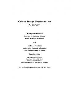
(a) Example Scene

(b) Visualization of a found segmentation

Figure 1: An example of a scene and a possible visualization of a found segmentation.

III. E VALUATION AND DATASETS A. Quality measures for evaluation A performance measure is a crucial part of any machine learning system. As users of a semantic segmentation system expect correct results, the accuracy is the most commonly used performance measure, but there are other measures of quality which matter when segmentation algorithms are compared. This section gives an overview of those quality measures. 1) Accuracy: Showing the correctness of the segmentation hypotheses is done in most publications about semantic segmentation. However, there are a couple of different ways how this accuracy can be displayed. One way to give readers a first qualitative impression of the obtained segmentations is by showing examples such as Figure 1. However, this can only support the explanation of particular problems or showcase special situation. For meaningful information about the overall accuracy, there are a couple of metrics how accuracy can be defined. For this section, let k ∈ N be the number of classes, nij ∈ N0 with i, j ∈ 1, . . . , k be the number of pixels whichPbelong to class i and were labeled as class j. Let k ti = j=1 nij be the total number of pixels of class i. One way to compare segmentation algorithms is by the pixel-wise accuracy of the predicted segmentation as done in many publications [SWRC06], [CP08], [LSD14].PThis is also called per-pixel rate and dek nii fined as Pi=1 . Taking the pixel-wise classification k i=1 ti accuracy has two major drawbacks: P1 Tasks like segmenting images for autonomous cars have large regions which have one class. This makes achieving classification accuracies of more than 30 % with a priori knowledge only possible. For example, a system might learn that a certain position of the image is most of the time “sky” while another position is most of the time “road”.

3

P2 The manually labeled images could have a more coarse labeling. For example, a human classifier could have labeled a region as “car” and the algorithm could have split that region into the general “car” and the more specific “wheel of a car” Three accuracy metrics which do not suffer from problem P1 are used in [LSD14]: Pn nii 1 • mean accuracy: k · i=1 ti • mean intersection over union: Pk 1 P nii i=1 ti + k nji −nii k · j=1 • frequency weighted intersection over union: Pk −1 P P ti nii ( p=1 tp ) i t + k n −n

segmentation, every image needs to be processed within 20 ms [BKTT15]. This time is called latency. Most papers do not give exact values for the time their application needs. One reason might be that this is very hardware, implementation and in some cases even data specific. For example, [HJBJ+ 96] notes that their algorithm needs 10 s on a Sun SparcStation 20. The fastest CPU ever produced for this system had 200 MHz. Comparing this directly with results which were obtained using an Intel i7-4820K with 3.9 GHz would not be meaningful. However, it does still make sense to mention the execution time as well as the hardware in individual papers. This gives the interested reader the possibility to i ii j=1 ji Another problem might be pixels which cannot be estimate how difficult it might be to adjust the algorithm assigned to one of the known classes. For this reason, to work in the required time-constraints. Besides the latency, the throughput is another [SWRC06] makes use of a void class. This class gets completely ignored for all quality measures. Hence the relevant characteristic of algorithms and implementatotal number of pixels is assumed to be width · height − tions for semantic segmentation. For example, for the automatic description of images in order to enable text number of void pixels. One way to deal with problem P1 and problem P2 search the throughput is of much higher importance is giving a confusion matrix as done in [SWRC06]. than latency. 3) Stability: A reasonable requirement on semantic However, this approach is not feasible if many classes segmentation algorithms is the stability of a segmenare given. The F -measure is useful for binary classifica- tation over slight changes in the input image. When tion task such as the KITTI road segmentation the image data is sightly blurred by smoke such as benchmark [FKG13] or crypt segmentation as done in Figure 4(c), the segmentation should not change. by [CRSS14]. It is calculated as “the harmonic mean Also, two images which show a slight change in perspective should also only result in slight changes in of the precision and recall” [PH05]: the segmentation [PH05]. tp Fβ = (1 + β)2 4) Memory usage: Peak memory usage matters (1 + β 2 ) · tp + β 2 · fn + fp when segmentation algorithms are used in devices like where β = 1 is chosen in most cases and tp means smartphones or cameras, or when the algorithms have true positive, fn means false negative and fp means to finish in a given time frame, run on the graphics false positive. processing unit (GPU) and consume so much memory Finally, it should be noted that a lot of other measures for single image segmentation that only the latest for the accuracy of segmentations were proposed for graphic cards can be used. However, no publication non-semantic segmentation. One of those accuracy were available mentioning the peak memory usage. measures is Normalized Probabilistic Rand (NPR) index which was introduced in [UPH05] and evalB. Datasets uated in [CSI+ 09] on dermoscopy images. Other The computer vision community produced a couple non-semantic segmentation measures were introduced in [MFTM01], but the reason for creating them seems to of different datasets which are publicly available. In be to deal with the under-defined task description of non- the following, only the most widely used ones as well semantic segmentation. These accuracy measures try to as three medical databases are described. An overview deal with different levels of coarsity of the segmentation. over the quantity and the kind of data is given by This is much less of a problem in semantic segmentation Table I. 1) PASCAL VOC: The PASCAL1 VOC2 challenge and thus those measures are not explained here. was organized eight times with different datasets: 2) Speed: A maximum upper bound on the execution Once every year from 2005 to 2012 [EVGW+ b]. time for the inference on a single image is a hard requirement for some applications. For example, in the 1 pattern analysis, statistical modelling and computational learning, case of autonomous cars an algorithm which classifies an EU network of excellence 2 Visual Object Classes pixel as street or no-street and thus makes a semantic

4

Training Beginning with 2007, a segmentation challenge was Prediction added [EVGW+ a]. The dataset consists of annotated photographs from Preprocessing Data www.flicker.com, a photo sharing website. There are augmentation multiple challenges for PASCAL VOC. The 2012 Feature extraction competition had five challenges of which one is a segmentation challenge where a single class label was given for each pixel. The classes are: aeroplane, bicycle, Window PostWindow-wise bird, boat, bottle, bus, car, cat, chair, cow, dining table, extraction Classification processing dog, horse, motorbike, person, potted plant, sheep, sofa, train, tv/monitor. Figure 2: A typical segmentation pipeline gets raw Although no new competitions will be held, new pixel data, applies preprocessing techniques algorithms can be evaluated on the 2010, 2011 and like scaling and feature extraction like HOG 2012 data via http://host.robots.ox.ac.uk:8080/ features. For training, data augmentation The PASCAL VOC segmentation challenges use the techniques such as image rotation can be segmentation over union criterion (see Section III-A). applied. For every single image, patches of 2) MSRCv2: Microsoft Research has published a the image called windows are extracted and database of 591 photographs with pixel-level annotation those windows are classified. The resulting of 21 classes: aeroplane, bike, bird, boat, body, book, semantic segmentation can be refined by building, car, cat, chair, cow, dog, face, flower, grass, simple morphologic operations or by more road, sheep, sign, sky, tree, water. Additionally, there complex approaches such as Markov Random is a void label for pixels which do not belong to Fields (MRFs). any of the 21 classes or which are close to the segmentation boundary. This allows a “rough and quick hand-segmentation which does not align exactly with IV. S EGMENTATION P IPELINE the object boundaries” [SWRC06]. 3) Medical Databases: The Warwick-QU Dataset consists of 165 images with pixel-level annotation of Typically, semantic segmentation is done with a 5 classes: “healthy, adenomatous, moderately differentiated, moderately-to-poorly differentiated, and poorly classifier which operates on fixed-size feature inputs differentiated” [CSM09]. This dataset is part of the and a sliding-window approach [DT05], [YBCK10], [SCZ08]. This means a classifier is trained on images Gland Segmentation (GlaS) challenge. The DIARETDB1 [KKV+ 14] is a dataset of 89 im- of a fixed size. The trained classifier is then fed with ages fundus images. Those images show the interior rectangular regions of the image which are called winsurface of the eye. Fundus images can be used to detect dows. Although the classifier gets an image patch of e.g. diabetic retinopathy. The images have four classes of 51 px × 51 px of the environment, it might only classify coarse annotations: hard and soft exudates, hemorrhages the center pixel or a subset of the complete window. and red small dots. This segmentation pipeline is visualized in Figure 2. 20 test and additionally 20 training retinal funThis approach was taken by [BKTT15] and a majordus images are available through the DRIVE data ity of the VOC2007 participants [EVGW+ a]. As this set [SAN+ 04]. The vessels were annotated. Addition- approach has to apply the patch classifier 512 · 512 = ally, [AP11] added vascular features. 262 144 times for images of size 512 px × 512 px, there The Open-CAS Endoscopic Datasets [MHMK+ 14] are techniques for speeding it up such as applying a are 60 images taken from laparoscopic adrenalectomies stride and interpolating the results. and 60 images taken from laparoscopic pancreatic Neural networks are able to apply the sliding window resections. Those are from 3 surgical procedures each. approach in a very efficient way by handling a trained Half of the data was annotated by a medical expert for network as a convolution and applying the convolution “medial instrument” and “no medical instrument”. All on the complete image. images were labeled by anonymous untrained workers to which they refer to as knowledge workers (KWs). However, there are alternatives. Namely MRFs and One crowd annotation was obtained for each image by Conditional Random Fields (CRFs) which take the a majority vote on a pixel basis of 10 segmentations information of the complete image and segment it in given by 10 different KWs. an holistic approach.

5

V. T RADITIONAL A PPROACHES the directions is calculated for each patch. HOG features Image segmentation algorithms which use traditional were proposed in [DT05] and are used in [BMBM10], approaches, hence don’t apply neural networks and [FGMR10] for segmentation tasks. 3) SIFT: Scale-invariant feature transform (SIFT) make heavy use of domain knowledge, are wide-spread feature descriptors describe keypoints in an image. The in the computer vision community. Features which can image patch of the size 16 × 16 around the keypoint be used for segmentation are described in Section V-A, is taken. This patch is divided in 16 distinct parts of a very brief overview of unsupervised, non-semantic the size 4 × 4. For each of those parts a histogram of segmentation is given in Section V-B, Random Decision 8 orientations is calculated similar as for HOG features. Forests are described in Section V-C, Markov Random This results in a 128-dimensional feature vector for Fields in Section V-E and Support Vector Machines each keypoint. (SVMs) in Section V-D. Postprocessing is covered in It should be emphasized that SIFT is a global feature Section V-G. for a complete image. It should be noted that algorithms can use combinaSIFT is described in detail in [Low04] and are used tion of methods. For example, [TNL14] makes use of a in [PTN09]. combination of a SVM and a MRF. Also, auto-encoders 4) BOV: Bag-of-visual-words (BOV), also called can be used to learn features which in turn can be used bag of keypoints, is based on vector quantization. by any classifier. Similar to HOG features, BOV features are histograms which count the number of occurrences of certain A. Features and Preprocessing methods patterns within a patch of the image. BOV are described The choice of features is very important in traditional in [CDF+ 04] and used in combination with SIFT approaches. The most commonly used local and global feature descriptors in [CP08]. features are explained in the following as well as feature 5) Poselets: Poselets rely on manually added extra dimensionality reduction algorithms. keypoints such as “right shoulder”, “left shoulder”, 1) Pixel Color: Pixel color in different image spaces “right knee” and “left knee”. They were originally (e.g. 3 features for RGB, 3 features for HSV, 1 feature used for human pose estimation. Finding those extra for the gray-value) are the most widely used features. A keypoints is easily possible for well-known image typical image is in the RGB color space, but depending classes like humans. However, it is difficult for classes on the classifier and the problem another color space like airplanes, ships, organs or cells where the human might result in better segmentations. RGB, YcBcr, HSL, annotators do not know the keypoints. Additionally, the Lab and YIQ are some examples used by [CRSS14]. keypoints have to be chosen for every single class. There No single color space has been proven to be superior are strategies to deal with those problems like viewpointto all others in all contexts [CJSW01]. However, the dependent keypoints. Poselets were used in [BMBM10] most common choices seem to be RGB and HSI. to detect people and in [BBMM11] for general object Reasons for choosing RGB is simplicity and the support detection of the PASCAL VOC dataset. by programming languages, whereas the choice of 6) Textons: A texton is the minimal building block the HSI color space might make it simpler for the of vision. The computer vision literature does not give a classifier to become invariant to illumination. One strict definition for textons, but edge detectors could be reason for choosing CIE-L*a*b* color space is that it one example. One might argue that deep learning techapproximates human perception of brightness [KP92]. niques with Convolution Neuronal Networks (CNNs) It follows that choosing the L*a*b color space helps learn textons in the first filters. algorithms to detect structures which are seen by An excellent explanation of textons can be found humans. Another way of improving the structure within in [ZGWX05]. 7) Dimensionality Reduction: High-resolution iman image is histogram equalization, which can be ages have a lot of pixels. Having one or more feature per applied to improve contrast [PAA+ 87], [RM07]. 2) Histogram of oriented Gradients: Histogram of pixel results in well over a million features. This makes oriented gradients (HOG) features interpret the image training difficult while the higher resolution might not as a discrete function I : N2 → { 0, . . . , 255 } which contain much more information. A simple approach maps the position (x, y) to a color. For each pixel, there to deal with this is downsampling the high-resolution are two gradients: The partial derivative of x and y. image to a low-resolution variant. Another way of Now the original image is transformed to two feature doing dimensionality reduction is principal component maps of equal size which represents the gradient. These analysis (PCA), which is applied by [COWR11]. The feature maps are splitted into patches and a histogram of idea behind PCA is to find a hyperplane on which all

6

feature vectors can be projected with a minimal loss of information. A detailed description of PCA is given by [Smi02]. One problem of PCA is the fact that it does not distinguish different classes. This means it can happen that a perfectly linearly separable set of feature vectors becomes not separable at all after applying PCA. There are many other techniques for dimensionality reduction. An overview and a comparison over some of them is given by [vdMPvdH09]. B. Unsupervised Segmentation Unsupervised segmentation algorithms can be used in supervised segmentation as another source of information or to refine a segmentation. While unsupervised segmentation algorithms can never be semantic, they are well-studied and deserve at least a very brief overview. Semantic segmentation algorithms store information about the classes they were trained to segment while non-semantic segmentation algorithms try to detect consistent regions or region boundaries. 1) Clustering Algorithms: Clustering algorithms can directly be applied on the pixels, when one gives a feature vector per pixel. Two clustering algorithms are k-means and the mean-shift algorithm. The k-means algorithm is a general-purpose clustering algorithm which requires the number of clusters to be given beforehand. Initially, it places the k centroids randomly in the feature space. Then it assigns each data point to the nearest centroid, moves the centroid to the center of the cluster and continues the process until a stopping criterion is reached. A faster variant is described in [Har75]. k-means was applied by [CLP98] for medical image segmentation. Another clustering algorithm is the mean-shift algorithm which was introduced by [CM02] for segmentation tasks. The algorithm finds the cluster centers by initializing centroids at random seed points and iteratively shifting them to the mean coordinate within a certain range. Instead of taking a hard range constraint, the mean can also be calculated by using any kernel. This effectively applies a weight to the coordinates of the points. The mean shift algorithm finds cluster centers at positions with a highest local density of points. 2) Graph Based Image Segmentation: Graph-based image segmentation algorithms typically interpret pixels as vertices and an edge weight is a measure of dissimilarity such as the difference in color [FH04], [Fel]. There are several different candidates for edges.

The 4-neighborhood (north, east, south west) or an 8neighborhood (north, north-east, east, south-east, south, south-west, west, north-west) are plausible choices. One way to cut the edges is by building a minimum spanning tree and removing edges above a threshold. This threshold can either be constant, adapted to the graph or adjusted by the user. After the edge-cutting step, the connected components are the segments. A graph-based method which ranked 2nd in the Pascal VOC 2010 challenge [EVGW+ 10] is described in [CS10]. The system makes heavy use of the multicue contour detector globalPb [MAFM08] and needs about 10 GB of main memory [CS11]. 3) Random Walks: Random walks belong to the graph-based image segmentation algorithms. Random walk image segmentation usually works as follows: Seed points are placed on the image for the different objects in the image. From every single pixel, the probability to reach the different seed points by a random walk is calculated. This is done by taking image gradients as described in Section V-A for HOG features. The class of the pixel is the class of which a seed point will be reached with highest probability. At first, this is an interactive segmentation method, but it can be extended to be non-interactive by using another segmentation methods output as seed points. 4) Active Contour Models: Active contour models (ACMs) are algorithms which segment images roughly along edges, but also try to find a border which is smooth. This is done by defining a so called energy function which will be minimized. They were initially described in [KWT88]. ACMs can be used to segment an image or to refine segmentation as it was done in [AM98] for brain MR images. 5) Watershed Segmentation: The watershed algorithm takes a grayscale image and interprets it as a height map. Low values are catchment basins and the higher values between two neighboring catchment basins is the watershed. The catchment basins should contain what the developer wants to capture. This implies that those areas must be dark on grayscale images. The algorithm starts to fill the basins from the lowest point. When two basins are connected, a watershed is found. The algorithm stops when the highest point is reached. A detailed description of the watershed segmentation algorithm is given in [RM00]. The watershed segmentation was used in [JLD03] to segment white blood cells. As the authors describe, the segmentation by watershed transform has two flaws: Over-segmentation due to local minima and thick watersheds due to plateaus.

7

C. Random Decision Forests Random Decision Forests were first proposed in [Ho95]. This type of classifier applies techniques called ensemble learning, where multiple classifiers are trained and a combination of their hypotheses is used. One ensemble learning technique is the random subspaces method where each classifier is trained on a random subspace of the feature space. Another ensemble learning technique is bagging, which is training the trees on random subsets of the training set. In the case of Random Decision Forests, the classifiers are decision trees. A decision tree is a tree where each inner node uses one or more features to decide in which branch to descend. Each leaf is a class. One strength of Random Decision Forests compared to many other classifiers like SVMs and neural networks is that the scale of measure of the features (nominal, ordinal, interval, ratio) can be arbitrary. Another advantage of Random Decision Forests compared to SVMs, for example, is the speed of training and classification. Decision trees were extensively studied in the past 20 years and a multitude of training algorithms have been proposed (e.g. ID3 in [Qui86], C4.5 in [Qui93]). Possible training hyperparameters are the measure to evaluate the “goodness of split” [Min89], the number of decision trees being used, and if the depth of the trees is restricted. Typically in the context of classification, decision trees are trained by adding new nodes until each leaf contains only nodes of a single class or until it is not possible to split further. This is called a stopping criterion. There are two typical training modes: Central axis projection and perceptron training. In training, for each node a hyperplane is searched which is optimal according to an error function. Random Decision Forests with texton features (see Section V-A6) are applied in [SJC08] for segmentation. In the [MSC] dataset, they report a per-pixel accuracy rate of 66.9 % for their best system. This system requires 415 ms for the segmentation of 320 px×213 px images on a single 2.7 GHz core. On the Pascal VOC 2007 dataset, they report an average per-pixel accuracy for their best segmentation system of 42 %. An excellent introduction to Random Decision Forests for semantic segmentation is given by [SCZ08]. D. SVMs SVMs are well-studied binary classifiers which can be described by five central ideas. For those ideas, the training data is represented as (xi , yi ) where xi is the feature vector and yi ∈ { −1, 1 } the binary label for training example i ∈ { 1, . . . , m }.

1) If data is linearly separable, it can be separated by a hyperplane. There is one hyperplane which maximizes the distance to the next datapoints (support vectors). This hyperplane should be taken: 1 minimize kwk2 w,b 2 s.t. ∀m i=1 yi · (hw, xi i + b) ≥ 1 | {z }

sgn applied to this gives the classification

2) Even if the underlying process which generates the features for the two classes is linearly separable, noise can make the data not separable. The introduction of slack variables to relax the requirement of linear separability solves this problem. The trade-off between accepting some errors and a more complex model is weighted by a parameter C ∈ R+ 0 . The bigger C, the more errors are accepted. The new optimization problem is: m X 1 minimize kwk2 + C · ξi w 2 i=1

s.t. ∀m i=1 yi · (hw, xi i + b) ≥ 1 − ξi Note that 0 ≤ ξi ≤ 1 means that the data point is within the margin, whereas ξi ≥ 1 means it is misclassified. An SVM with C > 0 is also called a soft-margin SVM. 3) The primal problem is to find the normal vector w and the bias b. The dual problem is to express w as a linear combination of the training data xi : w=

m X

αi yi xi

i=1

where yi ∈ { −1, 1 } represents the class of the training example and αi are Lagrange multipliers. The usage of Lagrange multipliers is explained with some examples in [Smi04]. The usage of the Lagrange multipliers αi changes the optimization problem depend on the αi which are weights for the feature vectors. It turns out that most αi will be zero. The non-zero weighted vectors are called support vectors. The optimization problem is now, according to [Bur98]: maximize αi

m X i=1

m

αi −

s.t. ∀m i=1 0 ≤ αi ≤ C m X s.t. αi yi = 0 i=1

m

1 XX αi αj yi yj hxi , xj i 2 i=1 j=1

8

4) Not every dataset is linearly separable. This problem is approached by transforming the feature vectors x with a non-linear mapping Φ into a higher dimensional (probably ∞-dimensional) space. As the feature vectors x are only used within scalar product hxi , xj i, it is not necessary to do the transformation. It is enough to do the calculation K(xi , xj ) = hxi , xj i

y7 y4 y1 x1

x4

x7 y2 x2

y8 y5 x5

x8 y3

y9 y6

x9

x6

x3

Figure 3: CRF with 4-neighborhood. Each node xi represents a pixel and each node yi represents a label.

This function K is called a kernel. The idea of never explicitly transforming the vectors xi to the higher dimensional space is called the kernel trick. gets labeled as shown in Figure 3. For example, a MRF which is trained on images of the size 224 px×224 pixel Common kernels include the polynomial kernel and gets the raw RGB values as features has KP (xi , xj ) = (hxi , xj i + r)p 224 224 · 3} + |224{z · 224} = 200 704 | ·{z of degree p and coefficient r, the Gaussian radial output input basis function (RBF) kernel random variables. Those random variables are condi−γkxi −xj k2 2 tionally independent, given their local neighborhood. 2σ KGauss (xi , xj ) = e These (in)dependencies can be expressed with a graph. and the sigmoid kernel Let G = (V, E) be the associated undirected graph of an MRF and C be the set of all maximal cliques in Ktanh (xi , xj ) = tanh(γhxi , xj i − r) that graph. Nodes represent random variables x, y and where the parameter γ determines how much edges represent conditional dependencies. Just like in influence single training examples have. he 4-neighborhood [SWRC06] and the 8-neighborhood 5) The described SVMs can only distinguish between are reasonable choices for constructing the graph. two classes. Common strategies to expand those Typically, random variables y represent the class of a binary classifiers to multi-class classification is single pixel, random variables x represent a pixel values the one-vs-all and the one-vs-one strategy. In the and edges represent pixel neighborhood in computer one-vs-all strategy n classifiers have to be trained vision problems segmentation problems where MRFs which can distinguish one of the n classes against are used. Accordingly, the random variables y live 2 all other classes. In the one-vs-one strategy n 2−n on 1, . . . , nr of classes and the random variables x classifiers are trained; one classifier for each pair typically live on 0, . . . , 255 or [0, 1]. of classes. The probability of x, y can be expressed as A detailed description of SVMs can be found 1 P (x, y) = e−E(x,y) in [Bur98]. Z SVMs are used by [YHRF12] on the 2009 and 2010 P −E(x,y) is a normalization term PASCAL segmentation challenge [EVGW+ 10]. They where Z = x,y e did not hand their classifier in to the challenge itself, called the partition function and E is called the energy but calculated an average rank of 7 among the different function. A common choice for the energy function is X categories. E(x, y) = ψc (x, y) [FGMR10] also used an SVM based method with c∈C HOG features and achieved the 7th rank in the 2010 PASCAL segmentation challenge by mean accuracy. It where ψ is called a clique potential. One choice for cliques of size two x, y = (x1 , x2 ) is [KP06] needs about 2 s on a 2.8 GHz 8-core Intel processor. ( +w if x1 6= x2 ψc (x1 , x2 ) = wδ(x1 , x2 ) = E. Markov Random Fields −w if x1 = x2 MRFs are undirected probabilistic graphical models which are wide-spread model in computer vision. The According to [Mur12], the most common way of overall idea of MRFs is to assign a random variable for inference over the posterior MRF in computer vision each feature and a random variable for each pixel which problems is Maximum A Posteriori (MAP) estimation.

9

Detailed introductions to MRFs are given by [BKR11], [Mur12]. MRFs are used by [ZBS01] and [MSB12] for image segmentation. F. Conditional Random Fields CRFs are MRFs where all clique potentials are conditioned on input features [Mur12]. This means, instead of learning the distribution P (y, x), the task is reformulated to learn the distribution P (y|x). One consequence of this reformulation is that CRFs need much less parameters as the distribution of x does not have to be estimated. Another advantage of CRFs compared to MRFs is that no distribution assumption about x has to be made. A CRF has the partition function Z: X Z(x) = P (x, y) y

and joint probability distribution P (y|x) =

1 Y ψc (yc |x) Z(x) c∈C

VI. N EURAL N ETWORKS FOR S EMANTIC S EGMENTATION Artificial neural networks are classifiers which are inspired by biologic neurons. Every single artificial neuron has some inputs which are weighted and sumed up. Then, the neuron applies a so called activation function to the weighted sum and gives an output. Those neurons can take either a feature vector as input or the output of other neurons. In this way, they build up feature hierarchies. The parameters they learn are the weights w ∈ R. They are learned by gradient descent. To do so, an error function — usually cross-entropy or mean squared error — is necessary. For the gradient descent algorithm, one sees the labeled training data as given, the weights as variables and the error function as a surface in this weight-space. Minimizing the error function in the weight space adapts the neural network to the problem. There are lots of ideas around neural networks like regularization, better optimization algorithms, automatically building up architectures, design choices for activation functions. This is not explained in detail here, but some of the mayor breakthroughs are outlined. CNNs are neural networks which learn image filters. They drastically reduce the number of parameters which have to be learned while being still general enough for the problem domain of images. This was shown by Alex Krizhevsky et al. in [KSH12]. One major idea was a clever regularization called dropout training, which set the output of neurons while training randomly to zero. Another contribution was the usage of an activation function called rectified linear unit:

The simplest way to define the clique potentials ψ is the count of the class yc given x added with a positive smoothing constant to prevent the complete term from getting zero. CRFs as described in [LRKT09] have reached top performance in PASCAL VOC 2010 [VOC10] and are also used in [HZCP04], [SWRC06] for semantic segmentation. A method similar to CRFs was proposed in [GBVdW+ 10]. The system of Gonfaus et.al. ϕReLU (x) = max(0, x) ranked 1st by mean accuracy in the segmentation task + of the PASCAL VOC 2010 challenge [EVGW 10]. Those are much faster to train than the commonly used An introduction to CRFs is given by [SM11]. sigmoid activation functions 1 ϕSigmoid (x) = −x G. Post-processing methods e +1 Post-processing refine a found segmentation and Krizhevsky et al. implemented those ideas and particiremove obvious errors. For example, the morphological pated in the ImageNet Large-Scale Visual Recognition operations opening and closing can remove noise. The Challenge (ILSVRC). The best other system, which opening operation is a dilation followed by a erosion. used SIFT features and Fisher Vectors, had a perforThis removes tiny segments. The closing operation is a mance of about 25.7 % while the network by Alex erosion followed by a dilation. This removes tiny gaps Krizhevsky et al. got 17.0 % error rate on the ILSVRCin otherwise filled regions. They were used in [CLP98] 2010 dataset. As a preprocessing step, they downsamfor biomedical image segmentation. pled all images to a fixed size of 256 px×256 px before Another way of refinement of the found segmentation they fed the features into their network. This network is by adjusting the segmentation to match close edges. is commonly known as AlexNet. This was used in [BBMM11] with an ultra-metric Since AlexNet was developed, a lot of different contour map [AMFM09]. neural networks have been proposed. One interesting Active contour models are another example of a example is [PC13], where a recurrent CNN for semantic post-processing method [KWT88]. segmentation is presented.

10

Another notable paper is [LSD14]. The algorithm presented there makes use of a classifying network such as AlexNet, but applies the complete network as an image filter. This way, each pixel gets a probability distribution for each of the trained classes. By taking the most likely class, a semantic segmentation can be done with arbitrary image sizes. A very recent publication by Dai et al. [DHS15] showed that segmentation with much deeper networks is possible and achieves better results. More detailed explanations to neural networks for visual recognition is given by [LKJ15].

(a) Lens Flare Image by [Hus07]

(b) Vignetting Image by [Man12]

(c) Smoke by cauterization Image by [GVSY13]

(d) Camouflage Image by [Kaf07]

VII. P OSSIBLE P ROBLEMS IN THE DATA FOR S EGMENTATION ALGORITHMS Different segmentation workflows have different problems. However, there are a couple of special cases which should be tested. Those cases might not occur often in the training data, but it could still happen in the productive system. I am not aware of any systematic work which examined the influence of problems such as the following. A. Lens Flare Lens flare is the effect of light getting scattered in the lens system of the camera. The testing data set of the KITTI road evaluation benchmark [FKG13] has a couple of photos with this problem. Figure 4(a) shows an extreme example of lens flare. B. Vignetting Vignetting is the effect of a photograph getting darker in the corners. This can have many reasons, for example filters on the camera blocking light at the corners. C. Blurred images Images can be blurred for a couple of reasons. A problem with the lenses mechanics, focusing on the wrong point, too quick movement, smoke or foam. One example of a blurred image is Figure 4(c), which was taken during an in vivo porcine procedure of diaphragm dissection. The smoke was caused by cauterization.

(e) Transparency

(f) Viewpoint

Figure 4: Examples of images which might cause semantic segmentation systems to fail.

2) Camouflage: Some objects, like animals in the wild, actively try to hide (see Figure 4(d) as an example). In other cases it might just be bad luck that objects are hard for humans to detect. This problem has two interesting aspects: On the one hand, the segmenting system might suffer from the same problems as humans do. On the other hand, the segmenting system might be better than humans are, but it is forced to learn from images labeled by humans. If the labels are wrong, the system is forced to learn something wrong.

D. Other Problems

3) Semi-transparent Occlusion: Some objects like drinking glasses can be visible and still leave the object behind them visible as shown in Figure 4(e). This is mainly a definition problem: Is the seen pixel the glass label or the smartphone label?

If the following effects can occur at all and if they are problems depends heavily on the problem domain and the used model. 1) Partial Occlusions: Segmentation systems which employ a model of the objects which should be segmented might suffer from partial occlusions.

4) Viewpoints: Changes in viewpoints can be a problem, if they don’t occur in the training data. For example, an image captioning system which was trained on photographs of professional photographers might not have photos from the point of view of a child. This is visualized in Figure 4(f).

11

R EFERENCES

VIII. D ISCUSSION Ohta et al. wrote [OKS78] 38 years ago. It is one of the first papers mentioning semantic segmentation. In this time, a lot of work was done and many different directions have been explored. Different kinds of semantic segmentation have emerged. This paper presents a taxonomy of those kinds of semantic segmentation and a brief overview of completely automatic, passive, semantic segmentation algorithms. Future work includes a comparative study of those algorithms on publicly available dataset such as the ones presented in Table I. Another open question is the influence of the problems described in Section VII. This could be done using a subset of the thousands of images of Wikipedia Commons, such as https://commons.wikimedia.org/wiki/Category:Blurring for blurred images. A combination of different classifiers in an ensemble would be an interesting option to explore in order to improve accuracy. Another direction which is currently studied is combining classifiers such as neural networks with CRFs [ZJRP+ 15].

[AM98]

[AMFM09]

[AP11]

[BBMM11]

[BJ00]

[BKR11] [BKTT15]

[BMBM10]

[Bur98] [BVZ01]

[CDF+ 04]

[CJSW01]

[CLP98]

M. S. Atkins and B. T. Mackiewich, “Fully automatic segmentation of the brain in mri,” Medical Imaging, IEEE Transactions on, vol. 17, no. 1, pp. 98–107, Feb. 1998. [Online]. Available: http://ieeexplore.ieee.org/xpls/ abs_all.jsp?arnumber=668699 P. Arbelaez, M. Maire, C. Fowlkes, and J. Malik, “From contours to regions: An empirical evaluation,” in Computer Vision and Pattern Recognition, 2009. CVPR 2009. IEEE Conference on. IEEE, Jun. 2009, pp. 2294–2301. [Online]. Available: http://ieeexplore.ieee.org/xpls/ abs_all.jsp?arnumber=5206707 G. Azzopardi and N. Petkov, “Detection of retinal vascular bifurcations by trainable v4-like filters,” in Computer Analysis of Images and Patterns. Springer, 2011, pp. 451–459. [Online]. Available: http://www.cs.rug.nl/~imaging/databases/ retina_database/retinalfeatures_database.html T. Brox, L. Bourdev, S. Maji, and J. Malik, “Object segmentation by alignment of poselet activations to image contours,” in Computer Vision and Pattern Recognition (CVPR), 2011 IEEE Conference on. IEEE, Jun. 2011, pp. 2225–2232. [Online]. Available: http://ieeexplore.ieee.org/xpls/ abs_all.jsp?arnumber=5995659 Y. Boykov and M.-P. Jolly, “Interactive organ segmentation using graph cuts,” in Medical Image Computing and Computer-Assisted Intervention– MICCAI 2000. Springer, 2000, pp. 276– 286. [Online]. Available: http://link.springer.com/ chapter/10.1007/978-3-540-40899-4_28 A. Blake, P. Kohli, and C. Rother, Markov random fields for vision and image processing. Mit Press, 2011. S. Bittel, V. Kaiser, M. Teichmann, and M. Thoma, “Pixel-wise segmentation of street with neural networks,” arXiv preprint arXiv:1511.00513, 2015. [Online]. Available: http://arxiv.org/abs/1511.00513 L. Bourdev, S. Maji, T. Brox, and J. Malik, “Detecting people using mutually consistent poselet activations,” in Computer Vision–ECCV 2010. Springer, 2010, pp. 168–181. [Online]. Available: http://link.springer.com/chapter/10.1007/ 978-3-642-15567-3_13#page-1 C. J. Burges, “A tutorial on support vector machines for pattern recognition,” Data mining and knowledge discovery, vol. 2, no. 2, pp. 121–167, 1998. Y. Boykov, O. Veksler, and R. Zabih, “Fast approximate energy minimization via graph cuts,” Pattern Analysis and Machine Intelligence, IEEE Transactions on, vol. 23, no. 11, pp. 1222–1239, 2001. [Online]. Available: http://ieeexplore.ieee.org/ xpls/abs_all.jsp?arnumber=969114 G. Csurka, C. Dance, L. Fan, J. Willamowski, and C. Bray, “Visual categorization with bags of keypoints,” in Workshop on statistical learning in computer vision, ECCV, vol. 1, no. 1-22. Prague, 2004, pp. 1–2. H.-D. Cheng, X. Jiang, Y. Sun, and J. Wang, “Color image segmentation: advances and prospects,” Pattern recognition, vol. 34, no. 12, pp. 2259–2281, 2001. C. W. Chen, J. Luo, and K. J. Parker, “Image segmentation via adaptive k-mean clustering and knowledge-based morphological operations with biomedical applications,” Image Processing, IEEE Transactions on, vol. 7, no. 12, pp. 1673–1683, Dec.

12

[CM02]

[COWR11]

[CP08]

[CRSS]

[CRSS14]

[CS10]

[CS11]

[CSI+ 09]

[CSM09]

[CXGS12]

[DHS15]

[DT05]

1998. [Online]. Available: http://ieeexplore.ieee.org/ xpls/abs_all.jsp?arnumber=730379 D. Comaniciu and P. Meer, “Mean shift: A robust approach toward feature space analysis,” Pattern Analysis and Machine Intelligence, IEEE Transactions on, vol. 24, no. 5, pp. 603–619, 2002. [Online]. Available: http://ieeexplore.ieee.org/xpl/ login.jsp?tp=&arnumber=1000236 C. Chen, J. Ozolek, W. Wang, and G. K. Rohde, “A pixel classification system for segmenting biomedical images using intensity neighborhoods and dimension reduction,” in Biomedical Imaging: From Nano to Macro, 2011 IEEE International Symposium on. IEEE, 2011, pp. 1649–1652. [Online]. Available: https://www.andrew.cmu.edu/ user/gustavor/chen_isbi_11.pdf G. Csurka and F. Perronnin, “A simple high performance approach to semantic segmentation.” in BMVC, 2008, pp. 1–10. [Online]. Available: http://www.xrce.xerox.com/layout/set/print/ content/download/16654/118653/file/2008-023.pdf A. Cohen, E. Rivlin, I. Shimshoni, and E. Sabo, “Colon crypt segmentation website.” [Online]. Available: http://mis.haifa.ac.il/~ishimshoni/ SegmentCrypt/Download.htm ——, “Memory based active contour algorithm using pixel-level classified images for colon crypt segmentation,” Computerized Medical Imaging and Graphics, Nov. 2014. [Online]. Available: http://mis.haifa.ac.il/~ishimshoni/SegmentCrypt/ Active%20contour%20based%20on%20pixellevel%20classified%20image%20for%20colon% 20crypts%20segmentation.pdf J. Carreira and C. Sminchisescu, “Constrained parametric min-cuts for automatic object segmentation,” in Computer Vision and Pattern Recognition (CVPR), 2010 IEEE Conference on. IEEE, 2010, pp. 3241–3248. ——, “Cpmc: Constrained parametric min-cuts for automatic object segmentation,” Feb. 2011. [Online]. Available: http://www.maths.lth.se/matematiklth/ personal/sminchis/code/cpmc/ M. E. Celebi, G. Schaefer, H. Iyatomi, W. V. Stoecker, J. M. Malters, and J. M. Grichnik, “An improved objective evaluation measure for border detection in dermoscopy images,” Skin Research and Technology, vol. 15, no. 4, pp. 444–450, 2009. [Online]. Available: http://arxiv.org/abs/1009.1020 L. P. Coelho, A. Shariff, and R. F. Murphy, “Nuclear segmentation in microscope cell images: a handsegmented dataset and comparison of algorithms,” in Biomedical Imaging: From Nano to Macro, 2009. ISBI’09. IEEE International Symposium on. IEEE, 2009, pp. 518–521. [Online]. Available: http://murphylab.web.cmu.edu/data M. D. Collins, J. Xu, L. Grady, and V. Singh, “Random walks based multi-image segmentation: Quasiconvexity results and gpu-based solutions,” in Computer Vision and Pattern Recognition (CVPR), 2012 IEEE Conference on. IEEE, 2012, pp. 1656–1663. [Online]. Available: http: //pages.cs.wisc.edu/~jiaxu/pub/rwcoseg.pdf J. Dai, K. He, and J. Sun, “Instance-aware semantic segmentation via multi-task network cascades,” arXiv preprint arXiv:1512.04412, 2015. N. Dalal and B. Triggs, “Histograms of oriented gradients for human detection,” in Computer Vision and Pattern Recognition, 2005. CVPR 2005. IEEE Computer Society Conference on,

vol. 1, June 2005, pp. 886–893 vol. 1. [Online]. Available: http://ieeexplore.ieee.org/xpls/ abs_all.jsp?arnumber=1467360 M. Everingham, L. Van Gool, C. K. I. [EVGW+ a] Williams, J. Winn, and A. Zisserman, “The PASCAL Visual Object Classes Challenge 2007 (VOC2007) Results,” http://www.pascalnetwork.org/challenges/VOC/voc2007/workshop/index.html. [Online]. Available: http://host.robots.ox.ac.uk: 8080/pascal/VOC/voc2007/index.html [EVGW+ b] ——, “The PASCAL Visual Object Classes Challenge 2012 (VOC2012) Results,” http://www.pascalnetwork.org/challenges/VOC/voc2012/workshop/index.html. [Online]. Available: http://host.robots.ox.ac.uk: 8080/pascal/VOC/voc2012/index.html [EVGW+ 10] M. Everingham, L. Van Gool, C. K. Williams, J. Winn, and A. Zisserman, “The pascal visual object classes (voc) challenge,” International journal of computer vision, vol. 88, no. 2, pp. 303–338, 2010. [EVGW+ 12] M. Everingham, L. Van Gool, C. K. I. Williams, J. Winn, and A. Zisserman, “Visual object classes challenge 2012 (voc2012),” 2012. [Online]. Available: http://host.robots.ox.ac.uk:8080/pascal/ VOC/voc2012/index.html P. F. Felzenszwalb, “Graph based im[Fel] age segmentation.” [Online]. Available: http: //cs.brown.edu/~pff/segment/ [FGMR10] P. F. Felzenszwalb, R. B. Girshick, D. McAllester, and D. Ramanan, “Object detection with discriminatively trained part-based models,” Pattern Analysis and Machine Intelligence, IEEE Transactions on, vol. 32, no. 9, pp. 1627–1645, 2010. [FH04] P. F. Felzenszwalb and D. P. Huttenlocher, “Efficient graph-based image segmentation,” International Journal of Computer Vision, vol. 59, no. 2, pp. 167–181, 2004. [Online]. Available: http://link.springer.com/article/10.1023/ B:VISI.0000022288.19776.77 [FKG13] J. Fritsch, T. Kuehnl, and A. Geiger, “A new performance measure and evaluation benchmark for road detection algorithms,” in International Conference on Intelligent Transportation Systems (ITSC), 2013. [Online]. Available: http://www.cvlibs.net/datasets/kitti/eval_road.php [GBVdW+ 10] J. M. Gonfaus, X. Boix, J. Van de Weijer, A. D. Bagdanov, J. Serrat, and J. Gonzalez, “Harmony potentials for joint classification and segmentation,” in Computer Vision and Pattern Recognition (CVPR), 2010 IEEE Conference on. IEEE, 2010, pp. 3280– 3287. [GRC+ 08] S. Gould, J. Rodgers, D. Cohen, G. Elidan, and D. Koller, “Multi-class segmentation with relative location prior,” International Journal of Computer Vision, vol. 80, no. 3, pp. 300–316, Apr. 2008. [GVSY13] S. Giannarou, M. Visentini-Scarzanella, and G.Z. Yang, “Probabilistic tracking of affine-invariant anisotropic regions,” Pattern Analysis and Machine Intelligence, IEEE Transactions on, vol. 35, no. 1, pp. 130–143, 2013. [Har75] J. A. Hartigan, Clustering algorithms. John Wiley & Sons, Inc., 1975. [HDT02] C. Huang, L. Davis, and J. Townshend, “An assessment of support vector machines for land cover classification,” International Journal of remote sensing, vol. 23, no. 4, pp. 725–749, 2002. [HHR01] S. Hu, E. Hoffman, and J. Reinhardt, “Automatic lung segmentation for accurate quantitation of volumetric x-ray ct images,” Medical Imaging, IEEE

13

[HJBJ+ 96]

[Ho95]

[Hus07]

[HZCP04]

[JLD03]

[Kaf07]

[KKV+ 14]

[KP92]

[KP06]

[KSH12]

[KWT88]

[LKJ15]

[Low04]

Transactions on, vol. 20, no. 6, pp. 490–498, Jun. 2001. A. Hoover, G. Jean-Baptiste, X. Jiang, P. J. Flynn, H. Bunke, D. B. Goldgof, K. Bowyer, D. W. Eggert, A. Fitzgibbon, and R. B. Fisher, “An experimental comparison of range image segmentation algorithms,” Pattern Analysis and Machine Intelligence, IEEE Transactions on, vol. 18, no. 7, pp. 673–689, Jul. 1996. [Online]. Available: http://ieeexplore.ieee.org/xpls/ abs_all.jsp?arnumber=506791 T. K. Ho, “Random decision forests,” in Document Analysis and Recognition, 1995., Proceedings of the Third International Conference on, vol. 1. IEEE, 1995, pp. 278–282. [Online]. Available: http://ect.bell-labs.com/who/ tkh/publications/papers/odt.pdf Hustvedt, “File:cctv lens flare.jpg,” Wikipedia Commons, Nov. 2007. [Online]. Available: https://commons.wikimedia.org/wiki/File: CCTV_Lens_flare.jpg X. He, R. Zemel, and M. Carreira-Perpindn, “Multiscale conditional random fields for image labeling,” in Computer Vision and Pattern Recognition, 2004. CVPR 2004. Proceedings of the 2004 IEEE Computer Society Conference on, vol. 2, Jun. 2004, pp. II–695–II–702 Vol.2. [Online]. Available: http://ieeexplore.ieee.org/xpl/ login.jsp?tp=&arnumber=1315232 K. Jiang, Q.-M. Liao, and S.-Y. Dai, “A novel white blood cell segmentation scheme using scale-space filtering and watershed clustering,” in Machine Learning and Cybernetics, 2003 International Conference on, vol. 5, Nov 2003, pp. 2820–2825 Vol.5. [Online]. Available: http://ieeexplore.ieee.org/ xpl/login.jsp?tp=&arnumber=1260033 L. Kaffer, “File:great male leopard in south afrikajd.jpg,” Wikipedia Commons, Jul. 2007. [Online]. Available: https://commons.wikimedia.org/wiki/File: Great_male_Leopard_in_South_Afrika-JD.JPG V. Kalesnykiene, J.-k. Kamarainen, R. Voutilainen, J. Pietilä, H. Kälviäinen, and H. Uusitalo, “Diaretdb1 diabetic retinopathy database and evaluation protocol,” 2014. [Online]. Available: http://www2.it.lut.fi/project/imageret/diaretdb1/ J. M. Kasson and W. Plouffe, “An analysis of selected computer interchange color spaces,” ACM Transactions on Graphics (TOG), vol. 11, no. 4, pp. 373–405, 1992. Z. Kato and T.-C. Pong, “A markov random field image segmentation model for color textured images,” Image and Vision Computing, vol. 24, no. 10, pp. 1103–1114, 2006. [Online]. Available: http://www.sciencedirect.com/science/ article/pii/S0262885606001223 A. Krizhevsky, I. Sutskever, and G. E. Hinton, “Imagenet classification with deep convolutional neural networks,” in Advances in neural information processing systems, 2012, pp. 1097–1105. M. Kass, A. Witkin, and D. Terzopoulos, “Snakes: Active contour models,” International journal of computer vision, vol. 1, no. 4, pp. 321–331, Jan. 1988. [Online]. Available: http: //link.springer.com/article/10.1007/BF00133570 F.-F. Li, A. Karpathy, and J. Johnson, “CS231n: Convolutional neural networks for visual recognition,” 2015. [Online]. Available: http://cs231n.stanford.edu/ D. Lowe, “Distinctive image features from scale-

invariant keypoints,” International Journal of Computer Vision, vol. 60, no. 2, pp. 91–110, 2004. [Online]. Available: http://dx.doi.org/10.1023/B% 3AVISI.0000029664.99615.94 A. Levin, A. Rav-Acha, and D. Lischinski, [LRAL08] “Spectral matting,” Pattern Analysis and Machine Intelligence, IEEE Transactions on, vol. 30, no. 10, pp. 1699–1712, 2008. [Online]. Available: http://ieeexplore.ieee.org/xpls/ abs_all.jsp?arnumber=4547428 L. Ladický, C. Russell, P. Kohli, and P. Torr, [LRKT09] “Associative hierarchical crfs for object class image segmentation,” in Computer Vision, 2009 IEEE 12th International Conference on, 2009, pp. 739–746. [Online]. Available: http://ieeexplore.ieee.org/xpls/ abs_all.jsp?arnumber=5459248 [LSD14] J. Long, E. Shelhamer, and T. Darrell, “Fully convolutional networks for semantic segmentation,” arXiv preprint arXiv:1411.4038, 2014. [Online]. Available: http://arxiv.org/abs/1411.4038 [MAFM08] M. Maire, P. Arbelaez, C. Fowlkes, and J. Malik, “Using contours to detect and localize junctions in natural images,” in Computer Vision and Pattern Recognition, 2008. CVPR 2008. IEEE Conference on, June 2008, pp. 1–8. [Online]. Available: http://ieeexplore.ieee.org/xpls/ abs_all.jsp?arnumber=4587420 [Man12] M. Manske, “File:randabschattung mikroskop kamera 6.jpg,” Wikipedia Commons, Dec. 2012. [Online]. Available: https://commons.wikimedia.org/wiki/File: Randabschattung_Mikroskop_Kamera_6.JPG [MBLAGJ+ 07] S. Maldonado-Bascon, S. Lafuente-Arroyo, P. GilJimenez, H. Gomez-Moreno, and F. LopezFerreras, “Road-sign detection and recognition based on support vector machines,” Intelligent Transportation Systems, IEEE Transactions on, vol. 8, no. 2, pp. 264–278, Jun. 2007. [Online]. Available: http://ieeexplore.ieee.org/xpls/ abs_all.jsp?arnumber=4220659 [MBVLG02] N. Moon, E. Bullitt, K. Van Leemput, and G. Gerig, “Automatic brain and tumor segmentation,” in Medical Image Computing and Computer-Assisted Intervention—MICCAI 2002. Springer, 2002, pp. 372–379. [MFTM01] D. Martin, C. Fowlkes, D. Tal, and J. Malik, “A database of human segmented natural images and its application to evaluating segmentation algorithms and measuring ecological statistics,” in Computer Vision, 2001. ICCV 2001. Proceedings. Eighth IEEE International Conference on, vol. 2. IEEE, 2001, pp. 416–423. [Online]. Available: http://ieeexplore.ieee.org/xpls/ abs_all.jsp?arnumber=937655 [MHMK+ 14] L. Maier-Hein, S. Mersmann, D. Kondermann, S. Bodenstedt, A. Sanchez, C. Stock, H. G. Kenngott, M. Eisenmann, and S. Speidel, “Can masses of non-experts train highly accurate image classifiers?” in Medical Image Computing and Computer-Assisted Intervention–MICCAI 2014. Springer, 2014, pp. 438–445. [Online]. Available: http://opencas.webarchiv.kit.edu/?q=node/26 [Min89] J. Mingers, “An empirical comparison of selection measures for decision-tree induction,” Machine Learning, vol. 3, no. 4, pp. 319–342, 1989. [Online]. Available: http://dx.doi.org/10.1023/A% 3A1022645801436 [MSB12] G. Moser, S. B. Serpico, and J. A. Benediktsson, “Markov random field models for supervised land

14

[MSC]

[MSR]

[Mur12] [OKS78]

[PAA+ 87]

[PC13]

[PH05]

[PS07]

[PTN09]

[PXP00]

[Qui86]

[Qui93] [RKB04]

[RM00]

cover classification from very high resolution multispectral remote sensing images,” in Advances in Radar and Remote Sensing (TyWRRS), 2012 Tyrrhenian Workshop on. IEEE, 2012, pp. 235– 242. [Online]. Available: http://ieeexplore.ieee.org/ xpl/login.jsp?tp=&arnumber=6381135 “Object class recognition image database.” [Online]. Available: http://research.microsoft.com/ vision/cambridge/recognition/ “Image understanding research data,” Microsoft Research. [Online]. Available: http://research.microsoft.com/en-us/projects/ objectclassrecognition/ K. P. Murphy, Machine learning: a probabilistic perspective. MIT press, 2012. Y.-i. Ohta, T. Kanade, and T. Sakai, “An analysis system for scenes containing objects with substructures,” in Proceedings of the Fourth International Joint Conference on Pattern Recognitions, 1978, pp. 752–754. S. M. Pizer, E. P. Amburn, J. D. Austin, R. Cromartie, A. Geselowitz, T. Greer, B. ter Haar Romeny, J. B. Zimmerman, and K. Zuiderveld, “Adaptive histogram equalization and its variations,” Computer vision, graphics, and image processing, vol. 39, no. 3, pp. 355–368, 1987. [Online]. Available: http://www.sciencedirect.com/science/ article/pii/S0734189X8780186X P. H. Pinheiro and R. Collobert, “Recurrent convolutional neural networks for scene parsing,” arXiv preprint arXiv:1306.2795, 2013. [Online]. Available: http://arxiv.org/abs/1306.2795v1 C. Pantofaru and M. Hebert, “A comparison of image segmentation algorithms,” Robotics Institute, p. 336, 2005. [Online]. Available: http://riweb-backend.ri.cmu.edu/ pub_files/pub4/pantofaru_caroline_2005_1/ pantofaru_caroline_2005_1.pdf A. Protiere and G. Sapiro, “Interactive image segmentation via adaptive weighted distances,” Image Processing, IEEE Transactions on, vol. 16, no. 4, pp. 1046–1057, 2007. [Online]. Available: http://ieeexplore.ieee.org/xpls/ abs_all.jsp?arnumber=4130436 N. Plath, M. Toussaint, and S. Nakajima, “Multiclass image segmentation using conditional random fields and global classification,” in Proceedings of the 26th Annual International Conference on Machine Learning. ACM, 2009, pp. 817–824. D. L. Pham, C. Xu, and J. L. Prince, “A survey of current methods in medical image segmentation,” Annual Review of Biomedical Engineering, vol. 2, no. 1, pp. 315–337, 2000, pMID: 11701515. [Online]. Available: http:// dx.doi.org/10.1146/annurev.bioeng.2.1.315 J. R. Quinlan, “Induction of decision trees,” Machine learning, vol. 1, no. 1, pp. 81–106, Aug. 1986. [Online]. Available: http://dx.doi.org/ 10.1023/A%3A1022643204877 ——, C4.5: Programs for Machine Learning, P. Langley, Ed. Morgan Kaufmann Publishers, Inc., 1993. C. Rother, V. Kolmogorov, and A. Blake, “Grabcut: Interactive foreground extraction using iterated graph cuts,” ACM Transactions on Graphics (TOG), vol. 23, no. 3, pp. 309–314, 2004. [Online]. Available: http://delivery.acm.org/10.1145/1020000/ 1015720/p309-rother.pdf J. B. Roerdink and A. Meijster, “The watershed transform: Definitions, algorithms and paralleliza-

[RM07]

[RMBK06]

[SAN+ 04]

[SCZ08]

[SJC08]

[SM11]

[Smi02]

[Smi04]

[SSA12]

[SUM+ 11]

[SWRC06]

[TNL14]

tion strategies,” Fundam. Inform., vol. 41, no. 1-2, pp. 187–228, 2000. J. Reynolds and K. Murphy, “Figure-ground segmentation using a hierarchical conditional random field,” in Computer and Robot Vision, 2007. CRV ’07. Fourth Canadian Conference on, May 2007, pp. 175–182. [Online]. Available: http://ieeexplore.ieee.org/xpls/ abs_all.jsp?arnumber=4228537 C. Rother, T. Minka, A. Blake, and V. Kolmogorov, “Cosegmentation of image pairs by histogram matching - incorporating a global constraint into mrfs,” in Computer Vision and Pattern Recognition, 2006 IEEE Computer Society Conference on, vol. 1, June 2006, pp. 993– 1000. [Online]. Available: http://ieeexplore.ieee.org/ xpls/abs_all.jsp?arnumber=1640859 J. Staal, M. D. Abràmoff, M. Niemeijer, M. Viergever, B. Van Ginneken et al., “Ridge-based vessel segmentation in color images of the retina,” Medical Imaging, IEEE Transactions on, vol. 23, no. 4, pp. 501–509, 2004. [Online]. Available: http://www.isi.uu.nl/Research/Databases/DRIVE/ F. Schroff, A. Criminisi, and A. Zisserman, “Object class segmentation using random forests.” in BMVC, 2008, pp. 1–10. [Online]. Available: http://research.microsoft.com/pubs/ 72423/Criminisi_bmvc2008.pdf J. Shotton, M. Johnson, and R. Cipolla, “Semantic texton forests for image categorization and segmentation,” in Computer vision and pattern recognition, 2008. CVPR 2008. IEEE Conference on. IEEE, Jun. 2008, pp. 1–8. [Online]. Available: http://ieeexplore.ieee.org/xpls/ abs_all.jsp?arnumber=4587503 C. Sutton and A. McCallum, “An introduction to conditional random fields,” Machine Learning, vol. 4, no. 4, pp. 267–373, 2011. [Online]. Available: http://homepages.inf.ed.ac.uk/csutton/ publications/crftutv2.pdf L. I. Smith, “A tutorial on principal components analysis,” Cornell University, USA, vol. 51, p. 52, 2002. B. T. Smith, “Lagrange multipliers tutorial in the context of support vector machines,” Memorial University of Newfoundland St. John’s, Newfoundland, Canada, Jun. 2004. D. Schiebener, J. Schill, and T. Asfour, “Discovery, segmentation and reactive grasping of unknown objects.” in Humanoids, 2012, pp. 71–77. [Online]. Available: http://h2t.anthropomatik.kit.edu/ pdf/Schiebener2012.pdf D. Schiebener, A. Ude, J. Morimotot, T. Asfour, and R. Dillmann, “Segmentation and learning of unknown objects through physical interaction,” in Humanoid Robots (Humanoids), 2011 11th IEEE-RAS International Conference on. IEEE, 2011, pp. 500–506. [Online]. Available: http://ieeexplore.ieee.org/ielx5/6086637/ 6100798/06100843.pdf J. Shotton, J. Winn, C. Rother, and A. Criminisi, “Textonboost: Joint appearance, shape and context modeling for multi-class object recognition and segmentation,” in Computer Vision–ECCV 2006. Springer, 2006, pp. 1–15. [Online]. Available: http: //link.springer.com/chapter/10.1007/11744023_1 J. Tighe, M. Niethammer, and S. Lazebnik, “Scene parsing with object instances and occlusion ordering,” in Computer Vision and

15

[UPH05]

[vdMPvdH09]

[VOC10] [WAH97]

[YBCK10]

[YHRF12]

[ZBS01]

[ZGWX05] [Zha12] [ZJRP+ 15]

Pattern Recognition (CVPR), 2014 IEEE Conference on. IEEE, 2014, pp. 3748–3755. [Online]. Available: http://ieeexplore.ieee.org/xpls/ abs_all.jsp?arnumber=6909874 R. Unnikrishnan, C. Pantofaru, and M. Hebert, “A measure for objective evaluation of image segmentation algorithms,” in Computer Vision and Pattern Recognition-Workshops, 2005. CVPR Workshops. IEEE Computer Society Conference on. IEEE, 2005, pp. 34–34. [Online]. Available: http://repository.cmu.edu/cgi/ viewcontent.cgi?article=1365&context=robotics L. J. van der Maaten, E. O. Postma, and H. J. van den Herik, “Dimensionality reduction: A comparative review,” Journal of Machine Learning Research, vol. 10, no. 1-41, pp. 66–71, 2009. “Voc2010 preliminary results,” 2010. [Online]. Available: http://host.robots.ox.ac.uk/pascal/VOC/ voc2010/results/index.html G.-Q. Wei, K. Arbter, and G. Hirzinger, “Automatic tracking of laparoscopic instruments by color coding,” in CVRMed-MRCAS’97, ser. Lecture Notes in Computer Science, J. Troccaz, E. Grimson, and R. Mösges, Eds. Springer Berlin Heidelberg, 1997, vol. 1205, pp. 357–366. [Online]. Available: http://dx.doi.org/10.1007/BFb0029257 Z. Yin, R. Bise, M. Chen, and T. Kanade, “Cell segmentation in microscopy imagery using a bag of local bayesian classifiers,” in Biomedical Imaging: From Nano to Macro, 2010 IEEE International Symposium on, Apr. 2010, pp. 125– 128. [Online]. Available: http://ieeexplore.ieee.org/ xpls/abs_all.jsp?arnumber=5490399 Y. Yang, S. Hallman, D. Ramanan, and C. C. Fowlkes, “Layered object models for image segmentation,” Pattern Analysis and Machine Intelligence, IEEE Transactions on, vol. 34, no. 9, pp. 1731–1743, Sep. 2012. [Online]. Available: http://ieeexplore.ieee.org/xpls/ abs_all.jsp?arnumber=6042883 Y. Zhang, M. Brady, and S. Smith, “Segmentation of brain MR images through a hidden Markov random field model and the expectationmaximization algorithm,” Medical Imaging, IEEE Transactions on, vol. 20, no. 1, pp. 45–57, 2001. [Online]. Available: http://ieeexplore.ieee.org/xpls/ abs_all.jsp?arnumber=906424 S.-C. Zhu, C.-E. Guo, Y. Wang, and Z. Xu, “What are textons?” International Journal of Computer Vision, vol. 62, no. 1-2, pp. 121–143, 2005. Z. Zhang, “Microsoft kinect sensor and its effect,” MultiMedia, IEEE, vol. 19, no. 2, pp. 4–10, Feb. 2012. S. Zheng, S. Jayasumana, B. Romera-Paredes, V. Vineet, Z. Su, D. Du, C. Huang, and P. H. Torr, “Conditional random fields as recurrent neural networks,” in Proceedings of the IEEE International Conference on Computer Vision, 2015, pp. 1529–1537. [Online]. Available: http://www.robots.ox.ac.uk/~szheng/ papers/CRFasRNN.pdf

G LOSSARY ACM active contour model. 6 BOV bag-of-visual-words. 5 CNN Convolution Neuronal Network. 5, 9 CRF Conditional Random Field. 4, 8, 9, 11 GPU graphics processing unit. 3 HOG histogram of oriented gradients. 5, 6, 8 ILSVRC ImageNet Large-Scale Visual Recognition Challenge. 9 MAP Maximum A Posteriori. 8 MR magnetic resonance. 2, 6 MRF Markov Random Field. 4, 8 PCA principal component analysis. 5 RBF radial basis function. 8 SIFT scale-invariant feature transform. 5 SVM Support Vector Machine. 4, 6–8

16

A PPENDIX A TABLES Database Colon Crypt DB DIARETDB1 KITTI Road MSRCv1 MSRCv2 Open-CAS Endoscopic Datasets PASCAL VOC 2012 Warwick-QU

Image Resolution (width × height) (302 px − 1116 px) × (349 px − 875 px) 1500 px × 1500 px (1226 px − 1242 px) × (370 px − 376 px) (213 px − 320 px) × (213 px − 320 px) (213 px − 320 px) × (162 px − 320 px) 640 px × 480 px (142 px − 500 px) × ( 71 px − 500 px) (567 px − 775 px) × (430 px − 522 px)

Number of Images

Number of Classes

389 89 289 240 591 120 2913 165

2 4 2 9 23 2 20 5

Channels 3 3 3 3 3 3 3 3

Data source [CRSS] [KKV+ 14] [FKG13] [MSR] [MSR] [MHMK+ 14] [EVGW+ 12] [CSM09]

Table I: An overview over publicly available image databases with a semantic segmentation ground trouth.