A Swarm-based Fuzzy Logic Control Mobile Sensor Network for Hazardous Contaminants Localization X. Cui, T. Hardin, R. K. Ragade, and A. S. Elmaghraby Computer Engineering and Computer Science Department University of Louisville, KY 40292 X0cui001,cthard01,rkraga01,
[email protected] Abstract In this paper, we describe a swarm-based fuzzy logic control (FLC) mobile sensor network approach for collaboratively locating the hazardous contaminants in an unknown large-scale area. The mobile sensor network is composed of a collection of distributed nodes (robots), each of which has limited sensing, intelligence and communication capabilities. An ad-hoc wireless network is established among all nodes, and each node considers other nodes as extended sensors. By gathering other nodes’ locations and measurement data, each node’s FLC can independently determine its next optimal deployment location. Simultaneously, by applying the three properties of the swarm behavior: separation, cohesion and alignment, the approach can ensure the sensor network attains wide regional coverage and dynamically stable connectivity. The simulation presented in this paper shows the swarm-based FLC mobile sensor network can achieve better performance and have higher fault tolerance in the event of partial node failures and sensor measurement errors.
1. Introduction When the contents of a hazardous material container are accidentally or intentionally released into an open area, the material will mix with the air to become an aerosol or vapor. The contaminant can be dispersed into the surrounding area with the flow of air [8,9]. The traditional approach of using an animal such as a dog for detecting, tracking and seeking odor sources cannot be used for locating highly fatal aerosols. Continued sampling and careful search of the entire suspected area by a professional human with adequate personal protective equipment could finally locate all of the aerosol emission sources, but such an
0-7803-8815-1/04/$20.00 '2004 IEEE
194
approach is not efficient in terms of time requirements, not to mention the risk to the human operators. In recent years, the threat of biological and chemical weapons technologies is increasing. Quick location and containment of hazardous vapor/aerosol emission sources to reduce casualties are essentially important. With today’s advanced technology, different kinds of mobile systems equipped with electrical vapor/aerosol-sensors have been investigated to locate hazardous material emission sources in a suspected area [8,10,12,14,17]. The electronic vapor/aerosol sensors used on this model mobile system could only provide gas concentration information about a very small area [10]. Further, the sensors usually cannot provide an instantaneous and precise measurement of the vapor/aerosol concentration because of the sensor’s long response time and even longer recovery time. However, the natural diffusion phenomena of gases and aerosols tend to spread in the environment inducing a concentration gradient that can be used as a clue for tracing emission sources [15]. This gradient phenomenon is very easily be impacted by airflow and geographical features of the environment [8,10]. Currently, most research focuses on investigation techniques for locating the sources by using a single robot [10,13]. Because of the spatial limitations of a single robot, few robotic systems have been developed that demonstrate the ability to carry out the source localization task in a large-scale area with unstructured environment. The increasing interest in distributed multiple robotic systems [1,2,20] indicates that employing multiple inexpensive, simple mobile robots (as opposed to a single expensive, complex mobile robot) could perform exploration tasks in a large-scale area more efficiently. In this paper, we provide a swarmbased fuzzy logic control (FLC) algorithm that integrates groups of low-cost robots, which are
equipped with limited-range communication ability and relatively inexpensive aerosol sensors. Each robot acts as a node in the mobile sensor network. The control algorithm is implemented on each individual node, and each node decides its action. Each node’s action is regulated by swarm behavior [11], a computational metaphor inspired by social insects. This paradigm, which has been demonstrated by flocks of birds, is an ideal model for solving problems in a distributed manner. Three basic control behavior properties of swarm behavior (separation, cohesion and alignment) [15] are used to ensure that the sensor network attains large region coverage and maintains dynamic ad hoc network connectivity between nodes. By using this ad hoc connectivity, all of the information obtained by any node can be utilized by the others. In this mobile sensor network, each node will consider other nodes with which it can communicate as its mobile extended sensors. By gathering the data from other nodes, a node can detect the remote environment‘s aerosol concentration that it cannot directly detect and use the location of the sensors to generate control commands to guide the robots in the likely direction of the aerosol gradient. However, characteristics of the vapor/aerosol in the environment reduce the precision of each node’s sensor. At the same time, some environmental effects, such as: lack of GPS signal, loss of line-of-sight between nodes and odometer error, may hinder a robot’s self-localization ability. The problem is further complicated by the possibility of a sensor or node failure at any time. All these factors render the information from one node, and by extension, the entire network, incomplete, uncertain, and approximate. The FLC algorithm in this paper allows for uncertain inputs, and generates finite commands to control node moves to their optimal deployment location. Because of the possibility that a node may be unable to gather information from all other nodes, the FLC allows dynamically varying inputs. Consequently, the fuzzy control rules are generated dynamically based on how many inputs are available to the FLC. The next section gives a brief overview of the emission source localization by robots. Section 3 sketches the architecture of the swarm-based FLC algorithm and describes the way that swarm behavior controller is implemented. The last two sections present a simulation experiment that evaluates the swarm-based FLC algorithm along with the results and conclusion.
195
2. Related work Most early research about hazardous aerosol detection was based on the cold-war scenario. Scientists were interested in discovering methods of protection from bio/chemical weapons attack in the battlefield setting. That includes soldier personal protective equipment, anti-biochemical and antinuclear vehicles and hazardous materials detection in a battlefield. In recent years, with the increasing accidental release of hazardous gases and the increased risk of bio/chemical terrorism, researchers have begun developing methods for preventing the diffusion of hazardous gases or aerosols into an urban or otherwise sensitive geographical area. This research moves in two directions. One research concept focuses on establishing the accurate boundary or perimeter of a dynamically changing hazardous material contaminated area for preventing human exposure or enabling evacuation from the dangerous area. Hardin et al. [9] presented a modified particle swarm algorithm for robotic mapping of an area contaminated by hazardous materials. Flanigan [6] proposed using passive infrared to remotely detect hazardous vapors. Another related area is odor source localization. This research focuses on the use of robots to efficiently detect, track and seek the odor source. Previous approaches using multiple robots for detecting gas or aerosol sources include spiral surge [8], gradient-seek [10] and bias random walk [12]. The gradient seek approach is the most commonly used approach in odor localization. The bias random walk approach can be considered as a variation of the gradient-seek technique. This set of techniques uses the natural phenomena of diffusion as a clue for tracing emission sources. A robot’s movement is dependent upon the temporal and spatial changes in aerosol concentration as sensed by the robot. An increase in the concentration along the robot’s path is called a positive gradient while a decrease is called a negative gradient. The robot will always try to move in a direction that will generate a positive gradient. However, an individual robot using this approach is easily susceptible to local maxima and plateaus of the aerosol concentration. The spiral surge approach breaks down the whole search task into three sub tasks: plume finding, plume traversal and source declaration [8]. In the plume finding stage, the robot will perform an initial outward spiral search pattern to allow the robot to contact the
odor. When a robot encounters an odor, the robot will sample the wind direction and move upwind searching for the odor source. The utilization of wind direction as the main control parameter of the robot’s direction restricts this approach to an environment where the geographical status is relatively simple and the wind direction is stable. The lack of collaboration in this approach restricts each robot to only local information about the environment, and the team can easily be trapped in local odor maxima and plateaus. This approach cannot prevent the robot from repeatedly searching the same area while other areas are left uninvestigated. The primary drawbacks of previous approaches are due to lack of collaboration between robot team members. Each robot can only make decisions based on the local information it sensed from surrounding environment. A complex, dynamic environment makes those approaches impossible to get an optimal or near optimal decision based on limited local information. A new control algorithm that makes all robots fully collaborative for decision making based on information exchange and fusion needs to be developed.
3. The swarm-based FLC algorithm description
communications capability in the swarm. Due to robot mobility, the ad-hoc network topology may change rapidly over time. A table-driven routing protocol [16] is used in the network for routing all messages. The robots in the system use an occupancy grid map [1,13,21] (Fig. 1) to represent the environment. Each cell in the grid map is a square block with a unique identity number. We assume each robot’s communication range can only cover cells adjacent to a robot’s current location. Upon initialization, the robots have no prior knowledge about the environment, each cell is labeled as un-explored and the concentration value is unknown.
Figure 1: The environment grid map and expansion cells
3.1. Assumptions In the swarm-based FLC algorithm, we envision that a hazardous gas container is vented to the atmosphere in a large-scale area. A swarm of robots is deployed into this suspected area to act as a mobile sensor network to search for the source. Each robot is a node of the sensor network and is equipped with an appropriate sensor. We assume the sensor cannot always read the correct concentration value and sensor errors are considered as a kind of random noise. Each robot is only equipped with a local wireless communicator such as WLAN [19]. Comparing the scale of the suspected area that the swarm of robots will explore, the local communication range is very small. Further, each robot can only communicate directly with its neighbors. No robot has global communication capability. However, each robot has the capability to forward data packets for each other over possible multi-hop paths to allow communication between robots otherwise out of direct wireless communication range. This enables the establishment of an ad-hoc wireless network for building global
196
3.2. Maintaining an ad hoc communication
network during exploration At the initial time, all robots are deployed near each other and an ad-hoc wireless network is established among all robots. Via the ad hoc network, each robot can collect the aerosol concentration value and other information from the other robots. After a robot completes the measurement of the aerosol concentration of its current cell, a swarm behavior controller that implemented on each robot will be used for planning the next target cell. To ensure wide coverage without overlapping or interference between robots, the separation property of the swarm behavior requires each robot avoid exploration of a cell occupied by other robot. Although all unexplored and unoccupied cells in the grid map can be chosen as the robot’s next target cell, moving to a cell without another robot in an adjacent cell could result in lost network communications. To maintain connectivity of the ad hoc network, the
cohesion property of the swarm behavior uses the gradual expansion algorithm [4] to control each robot’s movement. Each robot can only navigate to the “expansion cells” in the grid map. According to [4], a robot’s “expansion cell” is defined as the cell in the grid map that is unexplored and unoccupied. In the grid map, each expansion cell has at least one robot located in one of its eight adjacent cells. This keeps the robot in contact with the ad hoc network. In figure 1, robot A’s expansion cells are the unexplored cells surrounding other four robots. Robot A can keep connectivity with other robots by choosing any cell from its expansion cell list. However, to steer robot move towards emission source, a uniquely robot moving direction need to be generated by the fuzzy logic controller.
controller that was discussed in section 3.2. The behavior controller will find out the “expansion cell” that most suits the moving direction as the robot’s deployment location. The block diagram of one robot’s swarm-based FLC is shown in Figure 2. Each robot in the sensor network has one set of swarm-based FLC system. Each component in this FLC system is described in the following.
3.3 Fuzzy Logic Controller As we indicated previously, the characteristics of vapor/aerosol sensors and the environment make it easy to generate errors in contaminant concentration measurement and self-localization. In addition, faults are possible due to a failure of robots and/or sensors. The FLC endows each robot with the ability to make decisions despite those uncertainties [18]. In our approach, the swarm-based FLC is implemented on each robot and each robot uses its swarm-based FLC to generate the optimal deployment location. In the swarm-based FLC, each individual robot considers other robots in the network as sensors. The other robots’ locations and the contaminate concentration sensor’s reading values can be collected through the ad hoc network. The information will be used as the inputs of the swarm-based FLC to generate a crisp output, the robot’s optimal moving direction. This moving direction will be sent to the swarm behavior
197
Figure 3 Linguistic variables of robot location 3.3.1 Fuzzification. Fuzzification is defined as the mapping from a real-valued point to a fuzzy set [3]. The FLC system in this paper receives other robots’ information as the inputs of the FLC and the fuzzification module converts inputs into fuzzy linguistic variable inputs. There are 11 types of linguistic variables as inputs to the FLC: robots’ location angle related to the local robot
includes 8 subsets: Front Zero (FZ), Front Right (FR), Front Left (FL), Right (R), Left (L), Rear Zero (RZ), Rear Right (RR), Rear Left (RL) (Figure 3). The contaminant concentration that each robot’s sensor detected can be represented as: Low (L), Medium (M) and High (H).
MIN and MAX of the membership function may have different value at different time-steps. For example, let us denote the n robots in the hazardous contaminate source localization simulation as R0,R1..…Rn. Corresponding to each robot Ri, we have following equations:
S i = {s i , 0 , s i ,1 ,........s i ,i −1, s i ,i +1 .....s i ,n }
υ i = max ( S i ) λi = min ( S i )
(1)
Vector S i represents the sensor reading values that robot Ri gathered from other robots in the sensor network. We set υ i as the variable MAX and λi as the variable MIN of the concentration value fuzzy set membership function to convert vector S i into a (a)
respective fuzzy set. Each robot’s sensor concentration reading value ranges from 0 to 100. The nearer a robot is to the emission source, the higher the sensor reading value. The sensor’s reading value will reach 100 when the sensor and source locate at same grid cell. At the initial stage, the mobile sensor network’s location is far from the emission source. A typical vector of sensor reading case S i may look like:
S i = {0.6711, 0.7352, 2.041, 11.11, 0.8547, 2.863, 0.4878, 2.777, 0.4878, 0.3181}. To convert the crisp values in this vector into linguistic sets, the maximum value υ i =2.041 is defined as MAX and the minimum value λi =0.3181 (b) Figure 4 (a) Membership function of robot location angle set. (b) Membership function of contaminant concentration value set The set of a given robot’s location angles relative to the other robots and the reading values of each robot’s sensors are considered as fuzzy sets with triangular and trapezoidal membership functions. The membership function for the location angle set and robot moving direction set are shown in figure 4(a). The robot location angles range from –180 to +180. When a robot’s location angle is input in the fuzzification module, the linguistic variable sets can be generated according to this membership function. The concentration set membership is shown in figure 4(b). The MAX and MIN values in figure 4(b) equal the minimum value and maximum value of all sensors’ reading data that the robot collected from other robots at each time-step. Because of the mobility of the sensor network in the contaminated area, the
198
is defined as MIN. By using the membership function shape in figure 4(b), other element of the vector can be classified as H, M or L separately. However, at the final stage, the mobile sensor network’s location is nearer the emission source, all of the sensor reading values will be very high. A typical final stage vector may look like: S i = {46, 28, 24, 21.23, 33.33, 14, 25, 16.25, 85, 61}. At that time, the value λi =14 is defined as MIN and
υ i =85 is defined as MAX. Although the MAX and MIN value are variable at different time-steps, the shape of the membership functions are fixed initially. For the purpose of this paper, as shown in figure 4(b), the simulation defines fuzzy sets membership as follows: Low(L) is in the range [0,50%] Medium(M) is in the range [30,70%] High(H) is in the range [60,100%]
The ranges [0,100%] represent the range from lowest to the highest sensor reading value gathered by robot Ri at a given point in time. 3.3.2 Fuzzy inference engine. Fuzzy inference engine is used to generate fuzzy outputs by evaluating the fuzzy rules with the fuzzy inputs. The fuzzy rules may use an expert’s experience and control knowledge. These fuzzy rules are described in IFTHEN form and use the above linguistic variables. In this paper, the fuzzy inference engine need convert the input information into robot’s next movement direction. As we indicated in the previous section, the diffusion of aerosol in the contaminated area will induce a gradient phenomenon. A high concentration indicates a location near the source. The rules set should tend to steer all robots to the vicinity of the highest reported concentration. In our approach simulator, we use MATLAB® fuzzy logic toolbox to generate the FLC module. The fuzzy rules input in the MATLAB® FLC module are shown as follows: If concentration is HIGH and direction is FZ, move to FZ expansion cell. If concentration is HIGH and direction is FL, move to FL expansion cell. . . . If concentration is HIGH and direction is RR, move to RR expansion cell. 3.3.3 Defuzzification. The output of the fuzzy inference engine is a fuzzy set. The output is robot’s moving direction and its membership function is same as the location angle inputs shown in figure 4(a). In the MATLAB® fuzzy logic toolbox, there five methods are provided for defuzzification: 1) centroid of gravity method, 2) bisector of area method, 3) mean of maximum method, 4) smallest of maximum method and 5) largest of maximum method. Since the task of the FLC controller is steering the robot move toward highest reported concentration, in our MATLAB® FLC module, the center of gravity method [3] is used to get a crisp output to control the robot’s next moving direction. The robot’s swarm behavior controller uses other robots current location to find out all expansion cells the robot has and uses the moving direction generated by the FLC to define the expansion cell located on the path of the moving direction as the robot’s optimal deployment location.
199
4. Simulation Experiments We developed a simulation to evaluate the swarmbased FLC approach. The simulation describes the suspect area as a 300 x 300 two-dimensional grid. We initialized one source of aerosol at a randomly selected position in the grid. The following mathematical model is used for generating the concentration of each cell in the grid. m
C ( x , y ) = N ( x, y ) + K * ∑ { i =0
Pi ri 2
}
(2)
This equation gives the concentration C(x,y) that can be sensed at a point (x,y) on the grid in the presence of m sources. Pi is the aerosol release speed of the source Si . K is a constant. ri is the distance between the grid point (x,y) and the source Si. N(x,y) is the noise and environmental effect on the point (x,y). The random aerosol sensor detection error is introduced in this simulation. To simplify the simulation, we generate a random noise pattern on the 300*300 cell grid map that 20% cells’ concentration values in the grid map are impacted by a random value that ranges from -10 to 10. This noise grid map is applied on the aerosol concentration map that generated by eq.2. The possible contaminant distribution grid map is shown in Figure 5. The dark spot on the up right is the emission source. The concentration value in the center of the emission source is 100. According to eq.2, the farther a cell is from the emission source, the lower the concentration value of the cell. The dark dots on the picture are the random noise dots. In our scenario, there is a 20% possibility that a robot’s sensor cannot precisely measure the contaminant value. Instead, the sensor output a random value shown as the dark dot in figure 5. The dark line in the figure is the routing path of the mobile sensor network that locates the source in this environment by using our swarm-based FLC approach. We will explain more detail in section 5. The number of robots deployed in this simulated environment is 11. All robots can be randomly deployed in the grid, or they can be deployed based on the requirements of different approaches. The time for a robot to move from one cell (point) to its neighbor cell (point) equals 1 simulation time-step. The time that a robot consumed for sampling, measuring the concentration in each cell is a random number that ranges from 1 to 4 time-steps, and this number is unknown to the robot before it moves into its new cell.
The source is considered to be located only when a robot moves into the cell that the source located.
algorithm can still reach the source in a nearly optimal path.
5. Experiment Results 5.1 Evaluating the searching efficiency of the approach Two performance indicators are used for evaluating the performance of the approach: 1. The length of simulation time-steps for the robots to locate the emission source. 2. The distance between the source and the robot nearest to the source at each time step. The swarm-based FLC approach is implemented in the simulation and used for controlling 11 robots exploring the environment that has 20% random noise impact that we talked in section 4. For performance evaluation, we compared the swarm-based FLC approach with the gradient seek approach [10] in the same simulation environments. The swarm-based FLC approach and gradient seek approach are executed on the simulator 30 times separately. In Table 1, we present the results of the simulation. A paired-t test verifies with 99.9% confidence, that the FLC approach localizes the source faster than the Gradient Seek approach.
Figure 5 Location of the centroid of the sensor network at various simulation time steps.
5.2 Evaluating the approach’s tolerance on partial sensor failures
Table 1. Number of simulation steps required to localize the emission source. Mean Steps P N* Required to S.D. value Localize Source FLC 29 548.3 96.3 Gradient 29 1635.5 180.2 Difference -1087.2 204.2