A SYMBOLIC APPROACH TOWARDS CONSTRAINT BASED SOFTWARE VERIFICATION
SHUBHRA DATTA
Department of Computer Science
APPROVED:
Martine Ceberio, Ph.D.
Vladik Kreinovich, Ph.D.
Virgilio Gonzalez, Ph.D.
Benjamin Flores, Ph.D. Dean of the Graduate School
c
Copyright by Shubhra Datta 2011
to MY PARENTS and BIVAS ... with love
A SYMBOLIC APPROACH TOWARDS CONSTRAINT BASED SOFTWARE VERIFICATION
by
SHUBHRA DATTA, B.Tech.
THESIS Presented to the Faculty of the Graduate School of The University of Texas at El Paso in Partial Fulfillment of the Requirements for the Degree of
MASTER OF SCIENCE
Department of Computer Science THE UNIVERSITY OF TEXAS AT EL PASO
Acknowledgement First and foremost I offer my sincere gratitude to my supervisor, Dr Martine Ceberio, who has supported me throughout my thesis with her patience while allowing me the room to work in my own way. I am greatly indebted to her for my Masters degree without whose encouragement and effort this theses would be incomplete. I also thank the members of my graduate committee for their guidance and suggestions. I am heartily thankful to my fianc´ee Bivas Das for all his support and encouragement. Without his persuasion and guidance, I would not have come to study abroad in the first place. I also want to thank my dear friends Manali Chakraborty and Amritam Sarcar. They helped me in countless ways every time I needed them. Last but not the least, I thank my parents for supporting me throughout all my studies at UTEP, without their motivation and thoughtful decisions, I would not have been even what I am now. And finally, I offer my thanks and regards to all of those who supported me in any respect during the completion of the thesis.
Shubhra Datta NOTE: This thesis was submitted to my Supervising Committee on Sep 9, 2011. v
Abstract Verification and validation (V&V) are two components of the software engineering process that are critical to achieve reliability that can account for up to 50% of the cost of software development [20]. Numerous techniques ranging from formal proofs to testing methods exist to verify whether programs conform to their specifications. Recently, constraint programming techniques for V&V have emerged [15, 20]: they use the idea of proof by contradiction. They typically aim at proving that the code is inconsistent with the negation of the specification, which means that the software conforms to its specifications. Although the framework seems straightforward, the number of generated constraints can be high and the solving process tedious. In this work, we propose ideas for improvement based on symbolic manipulation of the constraints to be solved. Our approach differs from the current approach in its way to determine the compliance of the code with respect to its specification. Instead of using numeric solvers, we designed symbolic techniques to check compliance between the code and its specification. We analyzed how much practical the approach is if the program is correct and if the program is incorrect: can we make the verification process faster by applying our rules? CPBPV: a Constraint-Programming Framework for Bounded Program Verification [21], the work done by H. Collavizza, M. Rueher, and P. Hentenryck is the inspiration for our work. We established that our approach is feasible, and our experimental results prove that our proposed method is a promising addition to the existing framework to eliminate some of the basic challenges associated with constraint-based software verification.
vi
Table of Contents Page Acknowledgement . . . . . . . . . . . . . . . . . . . . . . . . . . . . . . . . . . . .
v
Abstract . . . . . . . . . . . . . . . . . . . . . . . . . . . . . . . . . . . . . . . . . .
vi
Table of Contents . . . . . . . . . . . . . . . . . . . . . . . . . . . . . . . . . . . . .
vii
List of Figures . . . . . . . . . . . . . . . . . . . . . . . . . . . . . . . . . . . . . .
x
1 Introduction . . . . . . . . . . . . . . . . . . . . . . . . . . . . . . . . . . . . . .
1
1.1
Motivation . . . . . . . . . . . . . . . . . . . . . . . . . . . . . . . . . . . .
1
1.2
What are we Proposing? . . . . . . . . . . . . . . . . . . . . . . . . . . . .
3
1.3
Thesis Outline . . . . . . . . . . . . . . . . . . . . . . . . . . . . . . . . . .
3
2 Preliminary Notions . . . . . . . . . . . . . . . . . . . . . . . . . . . . . . . . .
4
2.1
Verification, Validation, and Testing . . . . . . . . . . . . . . . . . . . . . .
4
2.2
Constraints . . . . . . . . . . . . . . . . . . . . . . . . . . . . . . . . . . .
5
2.2.1
General Definitions . . . . . . . . . . . . . . . . . . . . . . . . . . .
5
2.2.2
Kinds of Constraints . . . . . . . . . . . . . . . . . . . . . . . . . .
6
2.2.3
Constraint Programming and Solving . . . . . . . . . . . . . . . . .
7
Tree Exploration . . . . . . . . . . . . . . . . . . . . . . . . . . . . . . . .
9
2.3.1
Depth First Search (DFS) . . . . . . . . . . . . . . . . . . . . . . .
9
2.3.2
Bidirectional Search
. . . . . . . . . . . . . . . . . . . . . . . . . .
9
2.3.3
Weakest Precondition . . . . . . . . . . . . . . . . . . . . . . . . . .
11
3 Review of Related Research . . . . . . . . . . . . . . . . . . . . . . . . . . . . .
12
2.3
3.1
3.2
Existing Verification Techniques . . . . . . . . . . . . . . . . . . . . . . . .
12
3.1.1
Types of Verification . . . . . . . . . . . . . . . . . . . . . . . . . .
12
3.1.2
Techniques for Verification . . . . . . . . . . . . . . . . . . . . . . .
16
Related Research on Constraint Programming Techniques for Software Verification . . . . . . . . . . . . . . . . . . . . . . . . . . . . . . . . . . . . .
vii
21
3.2.1
Automatic Test Case Generation . . . . . . . . . . . . . . . . . . .
21
3.2.2
Conformity of Specifications and Code . . . . . . . . . . . . . . . .
23
3.2.3
Constraint Based Verification with Floating Point Numbers . . . . .
28
4 Limitations of Existing Approaches and Problem Statement . . . . . . . . . . .
32
4.1
Problem Statement . . . . . . . . . . . . . . . . . . . . . . . . . . . . . . .
32
4.1.1
Motivation for our approach . . . . . . . . . . . . . . . . . . . . . .
32
4.1.2
Limitations of CPBPV approach . . . . . . . . . . . . . . . . . . .
33
Our Approach . . . . . . . . . . . . . . . . . . . . . . . . . . . . . . . . . .
34
5 Design and Implementation . . . . . . . . . . . . . . . . . . . . . . . . . . . . .
37
4.2
5.1
Our Approach in a Nutshell . . . . . . . . . . . . . . . . . . . . . . . . . .
37
5.1.1
Inputs to Our Algorithm . . . . . . . . . . . . . . . . . . . . . . . .
37
5.1.2
Elements Used in Our Algorithm . . . . . . . . . . . . . . . . . . .
38
5.1.3
How the Algorithm Works . . . . . . . . . . . . . . . . . . . . . . .
39
5.2
Algorithm of Our Proposed Approach . . . . . . . . . . . . . . . . . . . . .
40
5.3
Our Approach in Detail . . . . . . . . . . . . . . . . . . . . . . . . . . . .
43
5.3.1
Specific Format of the Input Program . . . . . . . . . . . . . . . . .
43
5.3.2
Types of Constraints Generated . . . . . . . . . . . . . . . . . . . .
45
5.3.3
Types of Errors the Verifier can Catch . . . . . . . . . . . . . . . .
47
Examples . . . . . . . . . . . . . . . . . . . . . . . . . . . . . . . . . . . .
48
5.4.1
Absolute Difference Function
. . . . . . . . . . . . . . . . . . . . .
48
5.4.2
Insertion Sort Algorithm . . . . . . . . . . . . . . . . . . . . . . . .
50
5.4.3
Insertion Sort with Error . . . . . . . . . . . . . . . . . . . . . . . .
55
6 Experiments and Results . . . . . . . . . . . . . . . . . . . . . . . . . . . . . . .
56
5.4
6.1
Experiment Setup . . . . . . . . . . . . . . . . . . . . . . . . . . . . . . . .
57
6.2
Results . . . . . . . . . . . . . . . . . . . . . . . . . . . . . . . . . . . . . .
58
6.2.1
Experimental results for Goals 1 and 2 . . . . . . . . . . . . . . . .
58
6.2.2
Experimental Results for Goal 3 . . . . . . . . . . . . . . . . . . . .
68
7 Conclusion and Future Work . . . . . . . . . . . . . . . . . . . . . . . . . . . . .
71
viii
7.1
Conclusion . . . . . . . . . . . . . . . . . . . . . . . . . . . . . . . . . . . .
71
7.2
Future Work . . . . . . . . . . . . . . . . . . . . . . . . . . . . . . . . . . .
72
References . . . . . . . . . . . . . . . . . . . . . . . . . . . . . . . . . . . . . . . . .
74
Appendix Resources . . . . . . . . . . . . . . . . . . . . . . . . . . . . . . . . . . . . . . . . .
80
Curriculum Vitae . . . . . . . . . . . . . . . . . . . . . . . . . . . . . . . . . . . . .
81
ix
List of Figures 2.1
Depth First Search . . . . . . . . . . . . . . . . . . . . . . . . . . . . . . .
9
2.2
Bidirectional Search . . . . . . . . . . . . . . . . . . . . . . . . . . . . . . .
10
3.1
Verification , Validation and Testing
. . . . . . . . . . . . . . . . . . . . .
13
3.2
Problem with negation of constraints . . . . . . . . . . . . . . . . . . . . .
29
4.1
Simple example of how our Algorithm works . . . . . . . . . . . . . . . . .
36
5.1
STACK . . . . . . . . . . . . . . . . . . . . . . . . . . . . . . . . . . . . .
38
5.2
Tree for Absolute Difference Algorithm . . . . . . . . . . . . . . . . . . . .
51
5.3
Tree for Insertion Sort Algorithm . . . . . . . . . . . . . . . . . . . . . . .
54
6.1
correct sorting algorithms . . . . . . . . . . . . . . . . . . . . . . . . . . .
60
6.2
incorrect sorting algorithms . . . . . . . . . . . . . . . . . . . . . . . . . .
63
6.3
incorrect and correct sorting algorithms together . . . . . . . . . . . . .
65
6.4
RealPaver solution to the CSP generated from correct insertion sort al-
6.5
gorithm . . . . . . . . . . . . . . . . . . . . . . . . . . . . . . . . . . . . .
69
Verifier solution from correct insertion sort algorithm . . . . . . . . . . .
70
x
Chapter 1 Introduction 1.1
Motivation
Verification and validation (V&V) are two important aspects of software life-cycle and they play a key role to determine the reliability and quality of software. Software is heavily used in critical fields like air traffic control, medical diagnostics, space shuttle missions, stock market reporting etc. The presence of bugs in the software application can cause irreparable losses. There are several such catastrophic events which are caused by software failure such as, NASA Mars Climate Orbiter [51], a $125 million spacecraft, a key part of NASA’s Mars exploration program, crashed due to a mathematical mismatch that was not caught earlier. Northeast Blackout [36], costing $10 billion, happened due to a programming error which caused the failures occurred when multiple systems trying to access the same information. Ariane 5 [29], a space project built with $7 billion over 10 years, intended to give Europe overwhelming supremacy in the commercial space business, exploded in less than a minute due to a small computer program trying to stuff a 64-bit number into a 16-bit space. All these events clearly show that quality of software is of utmost importance and making sure the software meets the quality standards would have prevented these events. A report [51] says that “Software bugs are costing the U.S. economy an estimated $59.5 1
billion each year and improvements in testing could reduce this cost by about a third, or $22.5 billion”. Therefore it is very important to improve the V&V techniques in order to produce reliable and bug-free software. There exist different solving approaches to address software verification. In particular, the common verification techniques are: informal, static, dynamic, symbolic, formal, and constraint techniques [2]. Since informal techniques involve human intervention and reasoning, it is error prone. Since static techniques do not require machine execution of the model, they are sometimes unable to verify the execution behavior of the model. With dynamic analysis, it sometimes becomes very complex and sometimes the software is verified only partially for a particular test case (in the case of testing). Both symbolic and formal techniques involve very complex and costly mathematical analysis. Constraint verification techniques make use of assertions which can be difficult to state and place correctly in the code. Though the existing frameworks work reasonably well, there is still room for improvement: like cutting the cost or following a simpler approach. Recently, the CP (Constraint Programming) techniques constituted a new approach towards software verification and validation. The CP logic for V&V is reasonably simple and it is expected to be costeffective. CPBPV [21] is one of the most recent seminal works done in this field, proposed by H. Collavizza, M. Rueher and P. Hentenryck in 2010. This work has achieved significant performance improvement over the existing CP frameworks for V&V. The structure they follow to exploit the execution paths of the program, is very promising and if it can be successfully used in software verification, it can open a new direction in software industry. But their method has limitations: the number of generated constraints is very high, and as a result, the solution process is time consuming. In this work, we show how the computation time can be decreased.
2
1.2
What are we Proposing?
In the light of what we have discussed in motivation, in this work, we propose a framework similar to CPBPV in the structure but that only implements symbolic computations in inner nodes to detect any inconsistency earlier in the program. In the rest of the sections, we give the detailed analysis of our approach, and we show that this approach indeed reduces the computation time.
1.3
Thesis Outline
The rest of this thesis is organized as follows: In Chapter 2, the preliminary notions are presented. These include notions related to validation, verification and testing, constraints and tree search methods that we will be referring to in this work. In Chapter 3, a review of the related work is presented. We describe existing verification techniques, in particular constraint programming techniques. We also point out the pros and cons of using constraint-based techniques for V&V. In Chapter 4, we present our contribution. We first recall our problem statement and the motivation behind our approach, along with some simple pseudo code of the algorithm we are proposing. In Chapter 5, we go into the details of our proposed approach, explaining it with examples. Our experimental results are reported and analyzed in Chapter 6. Conclusions and directions for future work are presented in Chapter 7.
3
Chapter 2 Preliminary Notions In this thesis, the concepts of validation, verification, testing, constraints, weakest precondition, DFS tree traversal, bi-directional search and formal methods are central. In this chapter, we provide background notions on each of these topics.
2.1
Verification, Validation, and Testing
The concepts of validation, verification, and testing are closely related and even sometimes used interchangingly in the literature. The concepts of validation and verification are also used outside the programming world. In this section, we describe the meaning of these concepts as normally used and accepted in the programming world. Verification and validation are sometimes used together to refer to all the activities that we perform to check that software does what it is supposed to do. We adopt the definitions for validation and verification as they are used in software engineering. Verification refers to proving that a system satisfies its specification – usually proving that the code satisfies the design specifications [2]. In other words, when we verify, we ask the question: Are we building the product right? [50, 53]. Some of the verification techniques include inspections, walkthroughs, data flow analysis, debugging and testing. These are described in Section 3.1. Validation refers to checking that a system satisfies its specification – usually checking that the design specification satisfies the user’s requirements [2]. In other words, when we validate, we ask the question: Are we building the right product? [50, 53]. Some of the
4
activities carried out as part of validation are interviews and presenting prototypes to the customer to check that the design specification of the software meets his/her need. Testing means execution of a program or some parts of it. While testing a piece of the program, we should design test cases according to the specification of the program and run the test cases according to the specification of the program. We also have to run the test cases on the code. We have to observe the output and compares it with the expected output. We can say that the system has a failure if it fails a test case, i.e., the output does not coincide with the expected output. However, if the system passes a test case, i.e., the output does not coincide with the expected output, we cannot say that the program has been verified, we can only say that the system works for that specific test case [53].
2.2 2.2.1
Constraints General Definitions
Definition 1 (Constraint) Let D1 , . . . , Dn be sets. A constraint c over variables x1 ∈ D1 , . . . , xn ∈ Dn is a relation between its variables. By definition, a relation is a subset of the search space D1 ×. . .×Dn . Thus c restricts the possible combinations of values of the variables. A constraint solving problem consists of a finite set of variables, each defined on a non-empty domain, and a finite set of constraints restricting the values of the variables1 . More formally, Definition 2 (Constraint solving problem) A Constraint solving problem (CSP) is defined as a triple (C,X,D), where: • C is a set of constraints; • X = {x1 , . . . , xn } is the set of variables bound by the constraints of C; 1
A CSP can in some instances be completed with a cost function that measures the quality of the
assignments of the variables [47]
5
• D = D1 × . . . × Dn is the Cartesian product of the domains of the variables (xi ∈ Di ); it defines the initial search space. Definition 3 (Solution to a constraint) A solution of a constraint is an assignment of values to all variables, where these values are in the variables’ respective domains, in such a way that the constraint is satisfied. Definition 4 (Solution to a CSP) Solution of a CSP is an assignment of values to all variables, where these values are in the variables’ respective domains, in such a way that all constraints are satisfied.
2.2.2
Kinds of Constraints
In practice there are several types of constraints based on the nature of the constraints: • variables: There can be discrete and continuous constraints based on the domains of variables. For continuous constraints the domains are intervals or continuous ranges of possible values. As opposed to that, for discrete constraints, domains are discrete values for the variables. • symbolic expressions: e.g., linear and guarded constraints. These terms are described below. • expectations: e.g., global constraints, constrained local search etc. A global constraint is a constraint that captures a relation between a non-xed number of variables [48]. An example is the constraint alldifferent(x1 , . . . , xn ), which species that the values assigned to the variables x1 , . . . , xn must be pairwise distinct. Constrained local search is an example of an approach that searches over partial assignments that do not violate any constraints [48]. Rossi • solving approach: e.g., soft constraints. This term is explained below. 6
Here we review the most common ones in what follows. • Linear Constraints: This kind of constraints are of the form: a op b, where a and b are linear expressions and op ∈ {, ≤, ≥, =, 6=}. A linear expression consists of a numeric constant, the operator · that represents multiplication between two constants or a constant and a variable, and the binary operators − and + in infix notation. Linear constraints are used over the real, over the integers, or intervals. 6 · x − y ≥ 7 · y + z is an example of linear constraint. • Guarded Constraints: These constraints are of the form: condition → C where condition is a regular constraint or Boolean expression. A → B is a guarded constraint which behaves in the following way: • B is added to the set of constraints if A holds • B is discarded if A does not hold • A → B is suspended otherwise • Soft Constraints: These constraints may not be satisfiable. Their expression consists of regular constraints, but solving is different in a sense that the solutions of the constraints may not be found, and instead, only best tradeoffs achieved [2].
2.2.3
Constraint Programming and Solving
Constraint programming is a programming paradigm where the problem is stated in terms of the constraints or requirements and a solution for these constraints is found using a general or domain specific constraint solving method [6]. Table 2.1 is an example that shows a particular CSP [48] written in RealPaver syntax. RealPaver [31, 32] is a modeling language for numerical constraint solving. Table 2.2 shows the solution to the above CSP when solved using realpaver. 7
Table 2.1: Example of a CSP in RealPaver Variables int x in [-1000, 10000], int y in [-1000, 10000];
Constraints 4 ∗ x + 15 ∗ y = 750, 5 ∗ y + 7 ∗ y = 33;
Table 2.2: Solution to the above CSP using RealPaver INITIAL BOX x in [-1000, +10000] y in [-1000, +10000] OUTER BOX 1 x in [177.1874999999995, 177.1875000000005] y in [2.75, 2.750000000000001] precision: 9.09e−13 , elapsed time: 0 ms END OF SOLVING Property: reliable process (no solution is lost) Elapsed time: 0 ms
8
2.3
Tree Exploration
Since our approach is based on a tree structure of the program to verify, we describe hereafter tree traversal techniques that we will be using.
2.3.1
Depth First Search (DFS)
Depth first search (DFS) [22] is a technique for traversing or searching a tree structure starting at the root and exploring as far as possible along each branch in depth before backtracking when reaching a dead end (leaf or other) (See Fig. 2.1). 1
6 2
7
9
3 8 4
5
Figure 2.1: Depth First Search
Figure 2.1 shows the DFS traversal tree where the nodes in one branch are explored till the end of that branch. When one branch is explored, the possible branches that were left out during the initial exploration are considered one by one. Here the nodes are numbered in the order in which they are explored.
2.3.2
Bidirectional Search
The idea behind bidirectional search [16] is to run two simultaneous searches – one forward from the initial state another, backward from the goal state (see Fig. 2.2). The search
9
stops when searches from both directions meet in the middle. Once the search is over, the path from the initial state is then concatenated with the inverse of the path from the goal state to form the complete solution path. Initial State
Solution found at this point
Goal State
Figure 2.2: Bidirectional Search
If the tree expands with branching factor b and the distance from start to goal is d, time complexity of bidirectional search is O(bd/2 ) since each search needs only proceed to half the solution path. The advantage of bidirectional search is its speed. In order to implement bidirectional search a definite goal state is required. Also additional logic must be included to decide which search subtree to expand at each step. We can achieve noticeable speedup and improvement using this search if the following things can be guaranteed: • concrete information regarding goal state; • intersection between the two subtrees coming towards each other starting respectively from the start and goal state; and
10
• computational storage capability. It would be interesting to analyze the possible scope of improvement using this search technique integrated with our proposed approach. Though we did not address this issue in this work, we would like to do so in future.
2.3.3
Weakest Precondition
Weakest precondition approach works on a tree structure generated from the tree traversal of a program. We need to use weakest precondition while using bidirectional search technique, discussed in previous section. In [38], verification of programs based on weakest precondition strategy is proposed. Let us assume that we want to verify a program S where we know the postconditions R but not the precondition Q. We will denote this situation by {?}S{R}. There could be many arbitrary preconditions Q which are valid for the program S and the postcondition R. However, there is precisely one precondition describing the maximal set of possible initial states such that the execution of S leads to a state satisfying R. This Q is called the weakest precondition (A condition Q is weaker than P iff P ⇒ Q.)
11
Chapter 3 Review of Related Research In this chapter, we provide a review of the related research in the area of verification, validation and testing.
3.1
Existing Verification Techniques
In this section current approaches towards software verification and validation are described. In 1994, Balci [8] presented a taxonomy for the most common techniques for verification and validation where they are differentiated based on their degree of credibility and their common characteristics. Figure 3.1 shows the main classifications under verification, validation and testing. Then we also give a brief summary of Balci’s classification.
3.1.1
Types of Verification
Following are the main methods of verification: • Informal techniques. These techniques rely mainly on human reasoning and usually involve human participation. Some of the techniques that fit in this category are the following: – Audits: this technique requires one person whose goal is to find out the conformity of the software according to the established practices, standards, plans and guidelines [1, 8, 35]. – Inspections: they are usually done by a team with predefined roles; e.g., a reader, a recorder, a designer, a moderator, an implementer and a tester. An 12
Verification, Validation & Testing
Types of Verification
Existing Techniques
Informal - Audits - Inspections - Walkthroughs - Reviews
Symbolic - Path Analysis - Cause-Effect graphing - Partition Analysis - Symbolic Execution
Static - Data Flow Analysis - Structural Analysis - Graph-based Analysis - Syntax Analysis
Formal - Lambda Calculus - Predicate Calculus - Proof of Correctness Constraint - Assertion Checking - Inductive Assertions - Boundary Analysis
Dynamic - Execution Tracking - Debugging - Testing
Figure 3.1: Verification , Validation and Testing
inspection goes through several phases, such as overview of the model, fault finding process, faults resolution, examination of documents and it ensures that all faults are resolved [8]. Normally, an inspection consists of five phases: overview, preparation, inspection, rework, and follow-up [49]. – Walkthroughs: they are usually conducted by a team with members who are not directly involved in the development of the product, except for the model developer who is usually included as the only person who is also involved in the development process. The aim here is to show that a certain level of quality has been reached rather than analyzing code line-by-line to find faults [3, 25, 44, 45, 56]. – Reviews: they involve higher level techniques than inspections and walkthroughs. Like inspections, reviews are usually conducted by a team but it usually also includes managers. The objective here is to show to managers and sponsors that the product or software is being developed based on the specifica13
tions stated. In a review, models are also evaluated according to development standards, guidelines and objectives [8]. The main disadvantages of informal techniques are that, we may overlook some aspect of the program since informal techniques require human intervention and reasoning. It is human to err, therefore we may not reason correctly and miss errors that are present in the program. • Static Verification. They do not require execution of the model by machine. Some of the techniques that fall in this category are as follows; – Control Flow Analysis: This method is useful for identifying incorrect or inefficient constructs within model representation and it examines sequences of control transfers. A graph of the model is constructed in which nodes represent conditional branches and model junctions and links represent model segments between such nodes [11]. An edge represents the junction that assumes control, whereas a node of the model graph represents a logical junction where the flow of control changes. – Data Flow Analysis: This analysis assesses model accuracy with respect to the use of model variables [8]. This assessment is classified when variable space is allocated, accessed, and de-allocated [3]. This method is used to gather a program’s data flow without actually executing it. A data flow graph is constructed to aid in the data flow analysis. The nodes of the graph represent statements and corresponding variables. The edges represent control flow. Data flow analysis can be used to detect undefined or unreferenced variables and, when aided by model instrumentation, can track minimum and maximum variable values, data dependencies, and data transformations during model execution [4]. – Structural Analysis: It is performed to analyze the structure of the model or program. It usually constructs a control flow graph to analyze some features
14
about the program such as entry-exit points and use of unconditional branches [8]. Yucesan and Jacobson [57, 58] illustrated that modeling issues such as ambiguity of model specifications, state-accessibility, events-ordering, and execution stalling are problems for which general design techniques do not produce efficient solutions. They also showed that the problem of verifying structural properties of M&S applications (described in [58]) is difficult to solve. They proved it by applying the theory of computational complexity. – Cause-Effect Graphing: Causes and effects are first identified in the system being modeled and then their representations are examined in the model specification. It lists as many causes and effects as possible. Once the cause-effect graph has been constructed, a decision table is created by tracing back through the graph to determine combinations of causes that result in each effect. The decision table then is converted into test cases with which the model is tested [46, 55, 56]. – Syntax Analysis: This method ensures the correctness of the program with respect to the syntax rules of the programming language. It is normally done by the compiler [8, 11]. Static verification techniques are able to make some inferences about the semantics and some aspects of the execution of the model. Also they can verify the syntax of the program. But they are unable to verify the execution behavior of the model. Besides we need to show that the static verification tools (e.g., a compiler) is correct [55]. • Dynamic Verification. This technique is based on model execution. Following are some examples of this approach; – Execution Tracing: This technique generates trace data from the execution of the system line-by-line. The trace is then analyzed to find errors. But the
15
main problem is that the amount of trace produced is sometimes very large and complex. So it is very difficult to analyze [8]. – Debugging: This is the process of iteratively finding the errors that cause a system failure. Once the errors are found, we modify the system to correct the errors and keep debugging, until, ideally there are no errors, or commonly until we are satisfied with the system [8]. – Testing: This is one of the most commonly used V&V techniques. It first creates the test cases from the specification of a system and then runs the test cases. It decides whether the system failed or passed the test based on the output. A test case consists of a set of input data and a set of expected output. If the output does not coincide with the expected output then we can say that the system has a failure. However, if a system passes a test case then we can only say that the system works fine for that particular situation [53].
3.1.2
Techniques for Verification
Following are the techniques for verification: • Symbolic Verification. In this protocol, we run model with the symbolic inputs, given to it as inputs, which is translated throughout the execution path. The output consists of expressions that result from this transformation. Following are some of the techniques that fit in this category; – Path Analysis: We aim at testing all of the paths of a model in this technique. We often incorporate other techniques such as structural analysis and symbolic execution with this one. There can be different ways to choose test data according to the path coverage criteria that we want to achieve. Some of the coverage that we can achieve are: node coverage, multiple decision coverage,statement coverage, branch coverage and path coverage [55].
16
– Cause-Effect Graphing: This technique starts by identifying the causes and effects of the system. Then it constructs a cause-effect graph expressing the meaning of the system’s specifications. After that, it builds a decision table by considering possible combinations of causes that will cause each effect. Finally, we can build test-cases by considering the decision table [8, 52]. – Partition Analysis: This technique consists of three main steps. First, it partitions the model into sub models. And then, it compares the specification of the elements and their intended functionality of each sub model with the implementation of the elements and their actual functionality of each sub model. Finally, it produces test data to extensively test each sub model [55]. – Symbolic Execution: This technique involves executing the model with symbolic values as input instead of using actual values. Then the symbolic values (inputs to the model) are transformed during the execution of the model and at the end of the execution, the output consists of the resulting expression [55]. The main disadvantage of symbolic verification techniques is the process of deriving the symbolic expressions, which can be difficult and complex. These techniques are also costly in terms of human intervention in order to obtain or even interpret the symbolic results and the expressions [55]. • Formal Verification. Formal methods mean the use of mathematical and logical techniques to express, investigate, and analyze the specification, design, documentation, and behavior of both hardware and software. If attainable, formal methods are the most guaranteed way of doing model V&V. Formal verification is highly relevant to practical software engineering [13]. First it increases our understanding of the underlying nature of the program. Second, because of the proofs, engineers try to first check the consistency of the simplest implementation with requirements. This reduces errors and contributes the maintainability of error less programs. The most
17
commonly known techniques [37, 55] used in formal verifications are briefly described below followed by some existing verification methods : Techniques used in Formal Verification – Lambda Calculus: as described in [9], is a system for transforming the model into formal expressions by rewriting strings. Lambda calculus specifies rules for transforming the model into lambda calculus expressions. Using lambda calculus, the modeler can formally express the model so that mathematical proof of correctness techniques can be applied to it. A more details on types of lambda calculus can be found at [10]. – Predicate Calculus: as described in [7], provides rules for manipulating predicates, which are combinations of simple relations that can be either true or false. The model can be defined in terms of predicates and manipulated using the rules of predicate calculus. Predicate transformation [26] provides a basis for verifying model correctness by formally defining the semantics of the model with a mapping, which transforms model output states to all possible model input states. This representation provides the basis for proving model correctness. Some of the works based on predicate abstraction are given in [28, 54]. – Proof of Correctness: as described in [7, 49], corresponds to expressing the model in a precise notation and then mathematically proving that the executed model terminates and satisfies the requirements specification with sufficient accuracy. Attaining proof of correctness may not be possible using state of the art technology. However, the advantage of realizing proof of correctness is so great that when the capability is realized, it will revolutionize the model V&V. Formal Verification Methods – Hoare logic: Hoare used a very simple constructs for the language that has only assignment, sequencing of statements, if-then-else, and while [34]. Each of 18
these constructs is interpreted by a proof rule. All the rules are some forms of the expression {P }S{R}. Which means “if P is true before execution of S then provided S terminates R is also true”. The nature of the proof of a program S is as follows: The programmer supplies statements P and R, which supposedly describe the intended purpose of the program. Statement P defines properties of the input of the program; R defines properties of the output. Expression {P }S{R} is then the hypothesis to be proven. There have been some limitations: post-conditions are not easy to express in first-order logic. The proof of program in Hoare logic guarantees correctness of implementation only if the program is processed by a compiler based on Hoare logic. – Dijkstra’s approach: Dijkstra proposed the following two approaches: ∗ Weakest preconditions: This is described in Section 2.3. ∗ Parallel development of the program and the proof: Weakest preconditions are often associated with developing a program and its proof in parallel with the proof ideas guiding the program development [27]. – Mills’s functional correctness: Horlan Mills [42] has proposed a method of proof based on relations and functions rather than preconditions and postconditions. In this approach, programs or procedures are translated into functions relating outputs with inputs. This is the specification function. The proof is to demonstrate that the function computed from the program contains the specification function. There have been many arguments about feasibility of using formal verification. A proof has to convince its reader which, formal proof may fail to do. In the context of simultaneous development of an algorithm and a program, it can work very well for simple algorithms [7, 33] but some algorithms, like iteration schemas of numerical
19
analysis, are very difficult to deal with. So the emphasize is separating the proof of an algorithm from the proof of a program. The main disadvantage of formal verification techniques is that they require a formal mathematical proof of correctness. This can be very costly human-wise and machinewise and even it may not be possible with current technology. The main reasons include lack of adequate tools, lack of mathematical sophistication in developers, incompatibility with current techniques [40]. Though abstract data types provide an area in which the formal approach has been a success. Routine application of reasoning and data abstraction is just beginning in the industry [19], about 10-15 years after the initial research. • Constraint Verification. This technique verifies the software or the model based on the comparison of the assumptions made for the model to its actual behavior during the model execution. Some of the techniques that fit in this category are the following: – Assertion Checking: This technique places assertion statements in the code that should hold during the executionof the model or the program. It verifies the model or the program by comparing the information about the model on some state with its intended behavior at that state [55]. – Inductive Assertions: The inductive assertions technique involves writing input-output relations for all model variables. It places these relations at the beginning and the end of each path in the model. For each path, if the assertion at the beginning holds and all the statements in the path are executed then we can prove the correctness of the model or the program provided we prove the termination of the program or model. Though this technique is close to formal verification techniques, it has been included in constraint techniques because it makes use of assertions [55].
20
– Boundary Analysis: This method usually verifies the model’s behavior at boundaries of its input. Input is partitioned and test cases are generated with values inside the partition boundaries, on its boundaries and just past the boundary [55]. The main disadvantage of constraint verification techniques is that they make use of assertions which can be difficult to state and place correctly in the code. And also since stating assertions is tied to the formal specification, it also inherits the disadvantage and difficulty of formal specifications [55].
3.2
Related Research on Constraint Programming Techniques for Software Verification
In this section, researches on constraint-based software verification are presented in chronological order. Constraint solving for automated software verification and testing is an emerging topic. However, the extensive use of constraint programming in software verification is still being researched. To the best of my knowledge, Constraint Programming (CP) techniques have been studied and used in the V&V of software and hardware since the late 1980s - early 1990s. In [53], Waters proposed that the constraint modeling can be used as another approach for system validation (1991). The following section presents the history of constraint programming techniques being used for system validation.
3.2.1
Automatic Test Case Generation
The approach taken by Gotliebs et al. [30] consists of automatically generating test data that will execute a selected point in the code. They transformed the code into Static
21
Single Assignment1 (SSA) form and analyzed control-dependencies. Then they built a constraint system with this information and solved it. During solving the system, test data is generated in such a way that the selected point executes (if there is a feasible path that leads to the selected point). The main steps of Gotliebs et al. can be outlined as follows: 1. The first step involves translating the code into a constraint system from the SSA form and control-dependencies. 2. The resulting constraint system (CS) is a combination of constraints generated from the program and from the selected point. 3. The final step is to solve CS to generate the test data for the selected point if there exists at least one feasible path to the selected point. In [24], DeMillo and Offutt presented a constraint-based technique for automatically generating test data that causes a mutant program2 to fail (1991). Then in 1992, Chandra and Iyengar, presented a constrained-based approach to generate test cases to verify the designs of machines [17]. This approach is different from the previous one in a way that they generated test data to make a mutant program fail. Later in 1998, Michel Rueher from Universit´e de Nice-Sophia-Antipolis, France and Arnaud Gotlieb, Bernard Botella from Dassault Electronique, France introduced a new method for automatic test data generation based on constraint solving techniques. They translated a procedure into a constraint system by using SSA form and control dependencies. Then they solved the constraint system and checked if there was any feasible control flow path to execute a selected point in the program. If such a path existed, they generated test data that went through the path and executed the selected point. In addition, they also built a prototype implementation on a restricted subset of C language constructs [30]. 1
In compiler design, static single assignment form (often abbreviated as SSA form or simply SSA) is a
property of an intermediate representation (IR), which says that each variable is assigned exactly once [5]. 2 A mutant program is a program with a single modification to its original program.
22
Works done in [18] also showed that the constraint programming techniques have also been used to generate test data. But testing is not enough to verify the conformity between a software and its specifications. Since in testing, when the code satisfies all the test cases, we can only say that the code is valid for that particular test case. Therefor the code is partially correct. So we need other ways of verifying the code completely with respect to the specification.
3.2.2
Conformity of Specifications and Code
This section describes the work of Rueher et. al. in the context of proving the correctness of code with its specification. Collavizza and Rueher’s approach In [20] H´el`ene Collavizza and Michel Rueher explored the capabilities of CP techniques in software verification. Their approach handles only operations with integers, i.e., they work on discrete domains. The idea behind Collavizza’s and Rueher’s approach is that they transform the program and its specification into a constraint system. A program is verified if the union of the constraints derived from the program and the negation of constraints derived from the specification of the program is inconsistent, meaning the CSP does not have a solution. Let us assume that we have specification S and its implementation C: Then we solve C ∧ ¬S, which is in some sense similar to the process of resolution in logic. It shows that the implementation models the specification. That is, C |= S which is equivalent to C ∧ ¬S |=⊥.
The main steps of Collavizzas and Ruehers approach [20] can be outlined as follows: • Translate the program into a constraint system C. • Translate the negation of the specifications into a constraint system (¬S). 23
• Considering the conjunction of these two constraint systems as a CSP (possibly involving guarded constraints): C ∧ ¬S – If a solution is found, it means that the program does not meet its specification and the solutions to the CSP are the test cases that would fail to meet the specifications. – If a solution is not found, it means that the program meets its specification. In this work authors proposed to use a SAT solver first to deal with the disadvantage of the standard CSP solver. Example: Collavizza and Rueher’s Approach Here we consider the example given in [20], which is shown in algo 1. Algorithm 1 A method that returns the difference between two numbers Ensure: /** result ≥ 0 **/ 1:
function absolute(int i, int j)
2:
if (i < j) then
3:
return (j-i)
4: 5:
else return (i-j)
6:
end if
7:
end function When following the steps mentioned above, we get: 1. Translating the program into a constraint system: i < j → r = j − i, ¬(i < j) → r = i − j 2. Translating the negation of the specification into a constraint system: r < 0
24
3. Conjunction of these two constraint systems, give us the CSP: {i < j → r = j − i, ¬(i < j) → r = i − j, r < 0, Di = Dj = Dr = {0, . . . , 65535}}, where Di , Dj , Dr are the domains of the variables i,j, and r respectively. 0 to 65,535 is the range of short unsigned integeres. According to the verification approach proposed in [20], after translating the program and the negation of the specifications as a CSP, the CSP is solved and if it has no solution, it means that the program is correct with respect to the specifications, otherwise it means that the program does not meet the specifications. CPBPV: A Constraint-Programming Framework for Bounded Program Verification Their latest work in this field is CPBPV [21]. In this work they proposed a constraintprogramming framework for bounded program verification (CPBPV). The goal is to verify the conformity of a program with its specification that is to demonstrate that the specification is a consequence of the program. CPBPV generates constraint store from the specification and the program and explores execution paths non-deterministically. This non-determinism occurs while there is a conditional or iterative instruction and the nondeterministic execution refines the constraint store by adding constraints coming from conditions and from assignments. The input program is partially correct if each constraint so produced in the constraint store implies the post-condition. CPBPV does not explore spurious execution paths as it incrementally prunes execution paths early by detecting that the constraint store is not consistent. But it is important to notice that in order to verify the conformity between a program and its specification, CPBPV requires to check (explicitly or implicitly) all executables paths.
25
Example of CPBPV Approach Following is an example of the CPBPV verifier on binary search program (see algo 2) described in [21]. Algorithm 2 Binary Search Program Require: /** ∀ int i; i≥0 and i < t.length-1; t[i] ≤ t[i+1] **/ Ensure: /** (result != -1 → t[result] == v) && (result != -1 → ∀ int k; 0 ≤ k < t.length ;t[k] ! = v) **/ 1:
function binary-search(int[] t, int v)
2:
int l = 0
3:
int u = t.length-1
4:
while (l ≤ u) do
5:
int m = (l + u)/2
6:
if (t[m] == v) then return m
7: 8:
end if
9:
if (t[m] > v) then u = m-1
10: 11:
else l = m+1
12: 13:
end if
14:
end while
15:
return -1
16:
end function Assuming an array input of length 8, the initial constraint store (CS) is the precondition
cpre ≡ ∀0 ≤ i < 7 : t0 [i] ≤ t0 [i + 1] where t0 is an array of constraint variables capturing the input. CPBPV does SSA-like renaming [23] on the fly. Rest of the steps by the verifier are as follows:
26
• from line 2-3 add the constraints l0 = 0 ∧ u0 = 7. • since l0 ≤ u0 , enters loop body and add m0 = (l0 + u0 )/2 , which simplifies to m0 = 3. • line 6 is conditional statement giving rise to two alternatives and both must be explored. • taking the first alternative adds t0 [3] = v 0 to CS and executes line 7 which adds result = m0 to CS. • at this point CPBPV obtains an execution path p whose final constraint store cp is: cpre ∧ l0 = 0 ∧ u0 = 7 ∧ m0 = (l0 + u0 )/2 ∧ t0 [m0 ] = v 0 ∧ result = m0 . • CPBPV then checks whether this store cp implies the post-condition cpost by searching for a solution to cp ∧ ¬cpost . • If this test fails then this execution path satisfies the specification. • CPBPV then does the same thing with other alternatives from the conditional statement that were left out at the initial stage. Implementation Issues and Limitations Their prototype implementation uses a sequence of solvers(MIP, CP), where MIP is the mixed integer-programming tool ILOG CPLEX2 and CP is the constraint-programming tool Ilog JSOLVER. In order to very the constraints, MIP solver is called at each node of the executable paths. The CP solver is only called at the end of the executable paths when all the post conditions are considered. Also they use a depth-first strategy to traverse the executable paths of the code. According to our observation, the problem associated with CPBPV is they consider all executable paths and to check the conformity between the code and the specification they use interval solvers, which introduce noise and the solving process tedious. This work is
27
mostly what inspired us and we proposed an alternative symbolic approach following their work in order to avoid the constraint solving part.
3.2.3
Constraint Based Verification with Floating Point Numbers
In 2006, Blanc at el. [12] published their work on the verification and validation of programs with floating-point numbers (V3F). As part of the V3F project, the authors developed a constraint solver (FPCS) over floating-point numbers for the generation of test cases [12]. FPCS relies on two key techniques: Interval computation [43] and a computation of the inverse projection [41]. This project is now being continued in the Constraints and Proofs (CeP) team researching on subjects, such as software testing and verification, which can benefit from both constraint programming and proofs approaches. Techniques to solve constraints over the floating point numbers on the basis of projection functions can lead to slow convergence phenomena for very common constraints like addition and subtraction constraints. In [39], the authors have introduced new addition and subtraction constraints that can drastically speed up the filtering porcess. The work done in [12, 20] is the base of the work done in [15]. In this work, M. Ceberio, C. Acosta, and C. Servin proposed a way to handle floating-point numbers representing real values. Since SAT solvers are not efficient for such problems, they proposed an alternative approach so that there is no need for a SAT solver and it can be extended to handle domains of real numbers. The alternative they consider is the case of guarded constraints; they translate them by using the equivalence of logical implication with a disjunction. They discussed the process for solving constraints of the form A → B along with the pros and cons of it. Their proposed approach works as follows: • Translate the code (C) and the negation of the specifications (S) into constraints. • Translate constraints of the form A → B into ¬A ∧ B.
28
• Transform the CSP in the form of a CNF into a DNF CSP1 ∪ ... ∪ CSPm . • Solve the CSPs and consider the final solution to be: union of solutions of CSPi . Associated Challenges There are several challenges to the proposed method [15]: • Problem with negation of constraints: Since guarded constraints are converted to constraints involving negation, it may create problems for CSP solvers. These interval solvers may face two kinds of problems: the risk of false positives and missing solutions. These are explained in the following example. Example: Lets say we want to solve A∧¬B. We can solve by an outer approximation of A. In this case there are other areas get included in the solution (refer to the dark grey area of the left-hand-side picture of Fig. 3.2). We can also solve by an inner approximation of A. In this case some parts of solution are missed out (See Fig. 3.2).
Figure 3.2: Problem with negation of constraints
29
• Solving disjunction of CSPs: Since todays CSP solvers deal with intervals they produce lots of noise in the solution. Even CSPs that should have no solution might return solutions. • Problems to deal with Floating point numbers: – Absorption Floating-points are exposed to the problem of absorption. The following example (see Algo. 3) explains how this problem can be tricky to deal with. Algorithm 3 Example with floating point numbers 1: function foo() 2:
float x = 109 , y = 10−9 , z
3:
z = x+y
4:
if (z > x) then
5:
...
6:
end if
7:
if (z == x) then
8:
...
9:
end if
10:
end function The path conditions (z > x) can be easily extracted by the symbolic execution of the path 1 → 2 → 3 of program of example 2.2. Floating points are exposed to the problem of absorption. This occurs when we add a big floating point number with a very small one. Thus the step “z = x+y” gives 109 + 10− 9 = 109 , which activates the execution path 1 → 2 → 4, which leads to false results at the end. – Approximation
30
The real numbers is an infinite set. Since floating-points are approximation of real numbers, we cannot represent this infinite set in computer. Floating-point numbers are used to represent some of this real numbers.For example; the real number 1.00000045687 may not be represented as a floating-point number. – Poor arithmetical properties Addition and multiplication are neither associative (i.e., a+(b+c) 6= (a+b)+c) nor distributive (i.e., a*(b+c) 6= (a*b)+(a*c)) when floating-point numbers are involved. However they are commutative (i.e., b*c = c*b). Subtraction and division have the same properties as addition and multiplication. – Cancelation This is the problem with the floating-point numbers while subtracting two numbers that are close to each other. Throughout the computation on floating-point numbers, rounding errors may arise and they may be accumulated, hence, it may propagate and produce significant rounding errors. Considering the example given in [12], (10.00000000000004-10.0)/(10.000000000000004-10.0) results in 11.5 while it should be 10.0. These types of peculiarities make it difficult to handle floating point numbers while solving constraints involving them. These peculiarities can be handled by correctly designing the projection functions over floating-point intervals and by using a proper rounding mode [12].
31
Chapter 4 Limitations of Existing Approaches and Problem Statement In the previous chapter, we described the ongoing research in the fields of Constraint-based V&V and their associated challenges. Given the big picture of the problem in the context of constraint based V&V, we would like to highlight the problem statement and outline of our proposed approach to address some of these challenges.
4.1
Problem Statement
The objective in this research work is, given a specification and its corresponding implementation, to be automatically verify that the specification and the code are in compliance. The big picture is that we want to verify a code with respect to its specification provided we have the specification and an implementation. So we want to verify that an implementation meets its specification.
4.1.1
Motivation for our approach
Our approach is inspired by the logic described in CPBPV [21]. They used constraint store to represent both the code and its specification. In their approach they generate constraints from the code by non-deterministically exploring the execution path of the program. Whenever there is a conditional/iterative statement, they verify the constraint store produced so far with the specification. So they are calling the solvers at each decision
32
point and at the end with all the constraints generated. Our observation is that there are still scopes for improvement such as the following. • CPBPV creates a new variable each time the variable is assigned a new value which increases the constraint-store size. If the old variables are replaced with their new value then it helps to limit the constraint store size by not overpopulating it. • Doing some simple symbolic analysis to determine the compliance between the constraints and specification like updating a comparison constraint with an assignment constraint, string matching etc. • For sorting algorithms, it satisfies the specific loop invariants at each loop iteration. Since the complete set of specifications would not have been developed from any single loop iteration, the constraint store would be incomplete to check against specification at that point. So the big question is can we even decide that the constraints are consistent(or inconsistent) with the specification without really solving it? Here we want to consider an alternative way of how we can prove the effectiveness of the software without having to solve the constraints considering also the above mentioned factors.
4.1.2
Limitations of CPBPV approach
CPBPV has been shown to be efficient when we consider discrete domains such as in case of integers. However, its efficiency in the case of real numbers, to best of our knowledge, has not been analyzed. It seems possible but the risk of running into false positives is high. The authors also mentioned that in CPBPV verifier, it is critical to explore all execution paths and the main issue is how to effectively abstract memory stores by constraints and how to check satisfiability incrementally. Also they talked about hybridization of the CP technique and other verification technique being beneficial for V&V. At each step of the program, the constraint-store keeps on increasing with a high growth rate, which is then 33
sent to a solver. For a very complicated program, it could be very difficult in order to solve it. We want to consider an alternative approach so that it can reduce the growth of the constraint store produced from following the execution path of the program and also the need to consider a solver at each executable node is avoided.
4.2
Our Approach
We want to analyze a different approach where we do not use a solver at each decision point (conditional/iterative statement) and it is more symbolic in nature rather than actual constraint solving. In our approach, we try to symbolically detect the inconsistency by analyzing the constraints generated so far (either by direct implication or by derived implication from the constraint store). If there is any constraint which is opposing the specification rules then we stop exploring any more execution paths starting from that point, since those execution paths would be consequence of an invalid implementation logic. So we cut that branch and make a note of the depth of the tree at which the error was detected and how many nodes are generated so far. Then we start exploring the other alternatives from the conditional statement that were left out at the initial stage. In case the code is incorrect, we want to find out how much better our approach is in its way of detecting the inconsistency without using the solver. Following is a short pseudo code of our proposed approach with an example (see Algo. 4). Here S is the specification and STORE is the constraint store. And following is an example (see Fig. 4.1):
34
Algorithm 4 Pseudo code of our approach 1: for each line in code do 2:
STORE = STORE + [Constraints from line]
3:
if line is conditional/iterative statement then
4:
Verify STORE with S
5:
if STORE is consistent with S then Proceed
6: 7:
else Stop and start exploring other alternative branches
8: 9:
end if
10:
end if
11:
if Code End then
12:
Verify again
13: 14:
end if end for
35
/** @ensures Specification S **/ If A then B Else D
STORE = [ ] SPEC = S
Our Verifier
Verify STORE with S
if A if valid STORE then proceed yes
no
B
D
STORE = [neg(A),B ] SPEC = S
STORE = [A,B ] SPEC = S
Verify STORE with S
Verify STORE with S
Figure 4.1: Simple example of how our Algorithm works
36
Chapter 5 Design and Implementation In this chapter, we present the details of what we have proposed and implemented, and then we illustrate our approach with examples such as finding the absolute difference of two integer values as well as sorting algorithms such as insertion sort, bubble sort and selection sort
5.1
Our Approach in a Nutshell
Following we briefly describe the flow of our algorithm.
5.1.1
Inputs to Our Algorithm
Our algorithm needs the following two inputs in order to work: • The code: which is the program that needs to be verified with respect to its specification; • A well-defined specification of the input program: for example, for finding the absolute difference of two integer values, the requirement is that the difference must be greater than or equal to zero. So a well-defined specification is: result ≥ 0 where result is the difference between two values. For sorting algorithm for array length of 3, a well-defined specification is : a[1] ≥ a[0] ∧ a[2] ≥ a[1] where a is the array we want to sort.
37
5.1.2
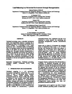
Elements Used in Our Algorithm
We used several notations to describe the variables used throughout our algorithm such as: • S: denotes the well-defined specification of the input program with which the verifier will tally the program. This is implemented as an array of string literals from the specification. • STORE: A repository which will hold the constraints generated from each line of input the program. This is also implemented as an array of strings. • VARSTORE: It stores the variables used in the input program with thier most recent values. This is implemented as a Hash Map where variables and their values are stored as a (key:value) pair. • STACK: This is to accommodate the alternative branches from an if condition, which are left out at initial stage and are explored later. Refer to figure 5.1. We used list data structure for this. if ( A ^ B)
A^B
~A
A ^ ~B
explored immediately will be explored later and we put them in STACK
STACK
A ^ ~B ~A
Figure 5.1: STACK
38
5.1.3
How the Algorithm Works
The verifier starts with the input program, its specification S, an empty constraint storeSTORE and an empty VARSTORE. It will start exploring the execution paths of the program starting with the first line of the code. For each line it keeps on generating the constraints and adds them to STORE until it encounters a conditional/iterative statement (also called decision point). The types of constraints that are generated from various type of program statement are discussed in section 5.3. The most important constraints are assignment and comparison constraints which are created from assignment and conditional statements respectively. We want to highlight the fact that each assignment constraint has an impact on the comparison constraints that comes later in the execution path. Suppose we have an assignment constraint like a[1] = val, and then the verifier sees a comparison constraint such as a[1] > 10. This comparison constraint will then be changed to val > 10. What the Algorithm does when there is a Conditional Statement It first generates all the possible branches from the conditional statement. For example, from a statement like if (j > 0&&a[j] > v) possible branches are if (j > 0&&a[j] > v), if (j 0&&a[j] 0&&a[j] > v), will be explored first and rest will be put into the STACK. It determines the consistency of the program traversed so far by validating the constraints in STORE with S which is done by the function CONSISTENT which is defined later in our algorithm. This consistency check is uniquely distinct than what is done in CPBPV. They call a solver at this stage to solve the CSP ST ORE ∧ ¬S. This involves a computationally tedious numerical solving of the CSPs which might incur noise and error in solution. Instead we do a simple symbolic analysis of the constraints in STORE with S.
39
Symbolic Verification Steps in Detail Each constraint in STORE is matched with each constraint in the set ¬S. For example, if S is r ≥ 0 then ¬S is r < 0. If there is any constraint in STORE which is r < 0 or there are set of constraints from which r < 0 can be derived, then the verifier detects that the STORE is inconsistent with S. It means that the execution path that it followed is an invalid implementation and it cuts that branch from the tree. Then it makes a note of that branch which is inconsistent. In case no constraint negates the S, the verifier proceeds through that branch for further processing. In case it cannot decide anything from the constraints with respect to the S then we can call a real solver to solve the CSP ST ORE ∧ ¬S. But we did not require the solver since the verifier was able to draw a strong conclusion. In case one branch is invalid, the verifier will look into the STACK since we do an exhaustive traversal of the search space. If the STACK is empty the verifier has completely traversed the whole tree. Otherwise it starts exploring the branches starting with the STACK top. What the Algorithm does at the Leaf Level When the verifier reaches the end of line of the input code or it sees a return statement, it is actually at the dead end for the branch it was working with. At the leaf level the constraints generated in constraint store is checked against the constraints generated from the negation of the specification like the way we described above. Following we give the layout of our algorithm.
5.2
Algorithm of Our Proposed Approach
First part of our algorithm is described in Algo 5 and the second part in Algo 6. Definition for function PROCESS is described in Algo 8. Definition for function CONSISTENT is described in Algo 7. 40
Algorithm 5 Algorithm Part 1 Require: /** The input program in specific format and a well-defined specification S **/ 1:
Translate the negation of the specification(¬S) into a constraint system
2:
while (Line is not the last line of the code and STACK 6= ∅) do
3: 4:
if (Line is conditional statement) then if (CONSISTENT(STORE,¬S)) then
. calls function CONSISTENT
5:
Generates all alternative branches from the if condition
6:
Follows only the true alternative among those branches
7:
if-condition ← PROCESS(if-condition,VARSTORE)
. calls function
PROCESS 8: 9:
Stores the other valid alternatives into a STACK for exploring them later else
10:
Detect an inconsistency and we note the depth at which it was found
11:
Stores the erroneous branch with depth and node count
12:
Looks into STACK for other possible unexplored branches
13:
Resumes execution starting with the branch at STACK TOP
14: 15:
end if else if Line is an assignment statement of the form ‘x = s’ then
16:
y ← PROCESS(s,VARSTORE)
17:
Variable x is assigned with value y
18:
The literal ‘x:y’ added to VARSTORE
. calls function PROCESS
41
Algorithm 6 Algorithm Part 2 19: else if (Line is the last line of the code/return statement) then if (CONSISTENT(STORE,¬S)) then
20:
. calls function CONSISTENT
Program is Verified
21:
else
22:
Stores the erroneous branch with depth and node count
23: 24:
end if
25:
Looks into STACK for other possible unexplored branches
26:
Resumes execution starting with the branch at the STACK TOP
27:
else if (Line is a loop statement of the form ‘LOOP1:’) then Stores the loop number and the line number for LOOP1
28: 29:
else if (Line is a goto statement of the form ‘GOTO LOOP1’) then
30:
Finds out the line number for LOOP1
31:
Resumes execution starting from that line
32:
end if
33:
end while
34:
if No erroneous branches found then . STACK is empty and all branches have been explored
35: 36:
Program is VERIFIED else
37:
Program is FAILED
38:
Prints the erroneous branches with the depth and node count
39:
Those branches are the test cases for which the program will fail
40:
end if
42
Algorithm 7 Algorithm to check consistency 1: function CONSISTENT(C, ¬S) 2:
Apply inference rules to simplify c
3:
for (Each literal s ∈ ¬S) do
. i > j, r = i − j will be simplified to r > 0)
for (Each Literal c ∈ C) do
4: 5:
if (s == c) then
6:
return 0
7:
Break
. Constraint c conforms to s which is a literal in ¬S set . 0 indicates not consistent
end if
8:
end for
9: 10:
end for
11:
return 1
12:
. c: constraint store, s: specification
. 1 indicates consistent
end function We discuss some of the details of our approach in the following section and then we
explain it with examples in the example section.
5.3
Our Approach in Detail
In the previous section we presented our algorithm. Here we will discuss some of the details of how our algorithm generates constraints from different types of program statements and the types of errors our verifier can detect symbolically starting with the specific format of the input program in order for the verifier to work.
5.3.1
Specific Format of the Input Program
At the beginning of our algorithm we have mentioned that the input code must be in a specific format in order for the verifier to work. For sorting algorithms we need to specify the array length on which the sorting algorithms will execute and a well-defined specification
43
Algorithm 8 Evaluates the right-hand-side of an assignment statement and returns the value 1: function PROCESS(s,v) 2: 3:
if s is of form ‘y’ then if ‘y:val(y)’ ∃ in VARSTORE then return val(y)
4: 5:
else return y
6: 7: 8: 9:
end if else if s is an arithmetic expression like ‘y+1’ then if ‘y:val(y)’ ∃ in VARSTORE then return val(y)+1
10: 11:
else return y+1
12: 13: 14: 15: 16: 17:
. s: string literal, v: VARSTORE
end if else if s is an array element of the form ‘a[i]’ then return ‘a[val(i)]’ else if s is an array element of the form ‘a[i+2]’ then return ‘a[val(i)+2]’
18:
end if
19:
end function
44
for all of the input programs. Also the input program must be a C program with the following specific format: • Function Declaration always followed by the starting curly brace. • IF condition must be in parenthesis and the statement must be followed by the starting curly brace. E.g. if (i < j){ of the IF block. • Block is always ended with the end curly brace in a separate line. • Loop Any loop statement is changed to the following format. Loop: if(A){ ... goto Loop; }
5.3.2
Types of Constraints Generated
Constraints are generated from each line of the code except the function definition. Types of constraints generated from the program statements and the actions taken by the verifier for each of these statements are as follows: (For a sample program please refer to algorithms in Examples section. • From Assignment statement: such as ‘x = y+1’ The above statement assigns value of y+1 to variable x. At this stage verifier also checks if x was declared initially or passed as function arguments; else it throws error ”variable x is used before declaration”. If it is declared, then it updates the value of x with value of y+1 in VARSTORE. For example, if y=0 then this constraint causes the value of x to be (0+1)=1.
45
• From Conditional statement: such as ‘if (i < l)’ The verifier first checks if (i < l) is valid by replacing the variables with their values. if it is invalid then it comes out of the if-block and continues execution starting after the block. If the condition is valid then a constraint (val(i) < val(l)) is added to STORE. At the same time the negation of the constraint which is (i ≥ l) is added to STACK only if (i ≥ l) is valid at that instant with values of i and l. For example, if i=0 and l=4 then (0 ≥ 4) is invalid and it is not added to the STACK. • From Loop statement: such as ‘Loop1’ Our verifier stores the loop number and the associated line number so that after each loop iteration it can restart execution for the next iteration starting from that line. • From Goto statement: such as ‘GOTO Loop1’ The verifier is set to the line at which Loop1 starts so that it can continue execution from that point. • From Else statement: ‘Else’ The Else is an alternative branch of a previous If statement. The verifier checks if the If branch is explored completely otherwise the Else is ignored. In case a complete execution path has been explored from the If, the verifier proceeds with the Elseblock. First it restores back the STORE as it was before the If block and then adds neg(If condition) to STORE which is retrived from STACK top. • From End brace: ‘}’ End Brace indicates end of a block or the program body. In case it is end of program body it means that a complete execution path has been explored. So at this point the verifier checks the consistency of the constraints in STORE which is generated from this execution path with the specification of the input program. If the execution
46
path is a valid one, the verifier then starts looking into the unexplored branches from the STACK that were left out during the previous stage.
5.3.3
Types of Errors the Verifier can Catch
While exploring the possible execution paths of the program we try to catch possible syntax errors from the code statements. Type of errors we are able to catch: • Variable declaration missing: If a variable is used in the program before it is declared, then the verifier throws this error. • Array index out of range: If array index is smaller than 0 or greater than array size, then the verifier throws this error. • Inconsistency detection: Following we explain the notion of inconsistency. No constraint in the constraint store should negate the specification, which is the requirement the code must satisfy in order to produce a correct end result. Example The specification for abs-diff function is result ≥ 0. So the negation of the specification will be result < 0. Now there should not be any constraint which is equal to result < 0 or set of constraints from which result < 0 can be derived in order to be consistent with the specification. According to the above definition, both of the following STOREs are invalid with respect to the specification result ≥ 0. – STORE = [result < 0]. This is a direct negation of the specification – STORE = [i < j, result = i − j]. From these constraints in STORE it can be derived thatresult < 0. Hence it negates the specification. The example here shows that we are doing symbolic analysis of the constraints generated from the code statements rather than directly solving the constraints as in 47
other CP techniques. According to[14] symbolic execution is a classical program testing technique which evaluates a selected control flow path with symbolic input data. The logic that we follow and its symbolic nature are illustrated with examples in the following section.
5.4
Examples
We tested our approach with numerical problems and the one we used is absolute difference function. Because of its simple nature it was easier to explain the symbolic nature of our algorithm with this. We have also used some sorting algorithms like insertion sort, selection sort and bubble sort. Following we explain our algorithms with these examples.
5.4.1
Absolute Difference Function
We have used the absolute difference algorithm described in algo 9 for our experiment. Algorithm 9 A method that returns the absolute difference between two numbers Ensure: /** result ≥ 0 **/ 1:
function absolute(int i, int j)
2:
if (i > j) then
3:
r =i−j
4: 5:
else r =j−i
6:
end if
7:
return r
8:
end function Let’s consider the program in Algo. 9 which returns the absolute difference between
two numbers. In this case, it is obvious that the returned result should be positive. So we define the specification as: (r >= 0), where r is the result.
48
Steps The parser in our program will do the following while it reads the above code line by line: 1. From function definition at line 1, Function Parameters i, j will be saved. 2. Steps for the if statement • First the verifier checks if variable i and l are declared. • Then it detects if the constraint generated so far, which is empty in this case, is consistent with the specification, r >= 0. It is consistent in this case. • Now it evaluates the expression i > j to see if it is a valid condition by putting the values ofi and j if available, if no numeric value is available for i and j which is the case here, it will just add the string literal i > j to STORE. • At the same time it will add i j] and VARSTORE:= r : i − j. From this the parser can derive the rule r > 0 and updates the STORE to [r > 0]. • It compares the constraints in the STORE with the specification which is r > 0 and it sees that the STORE is complying with it. So the program is consistent at this point. 49
• Then it restores back the STORE to what it was before if statement, since the if part is explored and validated. So STORE becomes ∅ since it was empty at the beginning of this if. • Then it goes to the STACK and pops the condition at STACK top which is i = 0, since they are not negating each other, so it satisfies the user defined specification and passes the verification step. 8. Since there is no more conditions in STACK to be explored, the verifier knows that the complete execution path from the input program is explored and then it declares that the Program is verified. 9. It will also give us the depth of tree traversal and the nodes generated during this tree traversal. Fig. 5.2 shows the tree generated from the traversal of the absolute-difference program.
5.4.2
Insertion Sort Algorithm
The previous example was a numerical problem in nature which shows how the symbolic verification steps work with this type of problems. So here we explain another example with sorting algorithm, which is symbolic in nature to show how the symbolic nature of our 50
Depth: 1 if ( i j
r=j-i
r=i-j
1
2
return r
return r
Figure 5.2: Tree for Absolute Difference Algorithm
verification logic will deal with it. The sorting algorithm we explained here is the insertion sort (Algo. 10). Though the verifier works for array length of more than 2, due to limited space we consider the insertion sort working on an array length of 2. After sorting the two elements the end result must satisfy this constraint a[0] v) do
9: 10:
a[j + 1] = a[j] j =j−1
11:
end while
12:
a[j + 1] = v
13:
i=i+1
14:
end while
15:
return a
16:
end function
52
STORE will have one comparison constraint a[0] > a[1] and VARSTORE will have v : a[1],a[1] : a[0], and a[0] = v. From the comparison and assignment constraints the parser derives the rule a[1] > a[0], which is then compared against the specification a[0] = 0 && a[j] 0= l => 0>=2
2
X
v = a[0] j = -1
3
Depth: 2 loop2: (j >= 0 && a[-1] > v) j >= 0 && a[-1] > v j >=0 && a[-1] 1= l => 1 >= 2
7
X
v = a[1] j=0
Depth: 4
8
loop2: (j >= 0 && a[0] > v) j >= 0 && a[0] < v j 2 < 2 loop2: (j >= 0 && a[-1] > v) j >= 0 && a[-1] > v i < l => 2 < 2
j >= 0 && a[-1]> v
12
X
X 13
14
a[0] = a[1] i=2 goto loop1
X 17
Depth: 6 loop1: ( i < l ) => 2 < 2 i < l => 2 < 2
X
return a
15
Depth: 7
Figure 5.3: Tree for Insertion Sort Algorithm
54
16
return a
18
5.4.3
Insertion Sort with Error
Here we illustrate the same insertion sort algorithm with an error. Let us change line 8 of Algo.10 to while(j ≥ 0 && a[j] < v) . Lets see how the verifier will detect the error even without calling the solver. Steps in Brief • The first iteration will generate STORE:= ∅ and VARSTORE:= v : a[0]. • From the second iteration for i = 1 the execution path will select < T5 , T8 , F8 > alternatives. So it will create STORE:= a[0] < a[1] and VARSTORE:= v : a[1], a[1] : a[0], a[0] = v. • After the third iteration where false alternative of the first if condition will be selected since i = 2 and l = 2 it goes to line 19 which is the return statement. Since this is the leaf level of that branch, the verifier checks the consistency. • Consistency check: At this point, STORE:= a[0] < a[1] and VARSTORE:= v : a[1], a[1] : a[0], a[0] = v. From the comparison and assignment constraints the parser derives the rulea[1] < a[0], which is then compared against the specification a[0] =a[1], a[0]>=a[2], a[1]>=a[2], a[2]=a[0], a[0]=a[2], a[1]=a[1], v=a[2], a[0]>=a[1], a[1]>=a[2];
INNER BOX 1 a[0] = 2 a[1] = 2 a[2] = 2 v =2 precision: 0, elapsed time: 0 ms
neg(SPEC)
INNER BOX 2 a[0] = 2 a[1] = 2 a[2] = 2 v =2 precision: 0, elapsed time: 0 ms END OF SOLVING Property: reliable process (no solution is lost) Elapsed time: 0 ms
Figure 6.4: RealPaver solution to the CSP generated from correct insertion sort algorithm
69
SPEC: a[0]a[1] or a[1]>a[2]
no This branch is consistent
Figure 6.5: Verifier solution from correct insertion sort algorithm
code is inconsistent with its specification while that is not the case for the correct insertion sort algorithm we have used. Therefore the numerical solver produced false positive in the solution. Using our approach, that is avoided and we could decide that the constraints in STORE has nothing common with the constraints from negation of the specification, hence the branch is correct. Overall, the experimental results above clearly show that our proposed logic works well to detect the consistency/inconsistency without using a solver and this simple logic if integrated with the existing framework can simplify the verification process by reducing the overhead associated with the constraint solving techniques.
70
Chapter 7 Conclusion and Future Work 7.1
Conclusion
Our aim is given a specification and an implementation of it, we want to verify the compliance between them. Though there exist many tools for conducting the software verification, none of them is really simple and cost-effective. Recently constraint programming techniques for software verification have emerged. CPBPV is the leading constraint-based framework for software verification. Though this tool works reasonably well, we observed that there exist areas for improvement as pointed out in Chapters 3 and 4. The CPBPV verifier provides significant gain in performance and functionalities compared to other tools for software verification. But the main overhead associated with CPBPV is its numerical constraint solving process using numerical solvers and an overflowing constraint store. The numerical solving process using a solver may produce noise and rounding errors due to floating point numbers in the solution. In this work we have come up with a different way of detecting the consistency between the program and its specification. We have followed a similar structure as CPBPV while exploring the execution paths from the program but we have used some simple symbolic steps instead of the numerical solving process while checking the compliance between the code and its specification. The symbolic step involves very simple form of string matching technique to see if there is any constraint generated so far, which is negating the specification. Also our logic reassigns new value to an existing variable without creating another one, which helps to restrict the constraint store size. We developed a new algorithm for checking the consistency between the code and its
71
specification symbolically instead of numerical constraint solving to reduce the overhead associated with the constraint programming technique for software verification. We have conducted experiments to show that our algorithm works well in deciding the consistency/inconsistency of the program with its specification without the aid of a numerical solver. We achieved a better performance while the input code is incorrect. With our symbolic verification steps we could catch errors faster than CPBPV. Our approach works on sorting algorithms for array length of 100 in the incorrect case while CPBPV does not: this is clearly an achievement over the existing constraint-based software verification frameworks and it shows the promise of our approach.
7.2
Future Work
Based on our experimental results, we observed that our algorithm: 1. takes exponential time with correct sorting algorithms for increasing array lengths. For correct sorting algorithms the verifier works till array length of 8. 2. does not handle very complex numerical expressions except simple arithmetic operations. 3. does not handle recursion and procedure calls and returns. 4. works with input program written in C and with some specific syntax as described in Section 5.3. Regardless of this limitation we have done much better than CPBPV with incorrect input codes and this improvement could be a potential addition to the existing state of the art technique for software verification. Here we describe how we are going to address the shortcomings listed above. 1. Currently the verifier takes exponential time for sorting algorithms when it works with array length of greater than 8. In order to address the timing issue, we want to 72
integrate the bi-directional search and weakest precondition strategy towards finding a solution with our framework. In bi-directional search, we start traversing from the start node and goal node simultaneously. So it reduces the time complexity in best case when these two paths intersect in the midway. But also when they do not intersect then we traverse the whole tree twice one starting from the top and another starting from the goal node. We want to find out the feasibility of this approach in our future work. 2. The verifier works with simple numerical expressions. There is an in-built function which processes arithmetic expressions, and it can be very easily upgraded in order to process complex arithmatic expressions. 3. To handle recursion and function calls, we will have to integrate modular verification techniques in our approach which we will address in future. 4. The parser in our verifier is written to identify specific types of program statements. This logic can be easily modified to identify more general program structures. Here are possible extensions to our work: • Catching as many types of errors as possible like infinite loop, type checking etc. • We would also like to explore the possibilities of integrating our work in the existing frameworks for software verification to analyze the performance and efficiency of the integrated model.
73
References [1] IEEE standards for Software Reviews and Audits. IEEE Computer Society, June 1989. www.cs.ucf.edu/ workman/cen5016/IEEE1028.pdf. [2] C. Acosta. A Constraint-based Approach to Verification of Programs with FloatingPoint numbers. Master’s thesis, The University of Texas at El Paso, December 2007. [3] W. R. Adrion, M. A. Branstad, and J. C. Cherniavsky. Validation, Verification, and Testing of Computer Software. Computing Surveys, 14(2):159–192, 1982. [4] F. E. Allen and J. Cocke. A Program Data Flow Analysis Procedure. Communications of the ACM, 19(3):137–147. [5] A. W. Appel. Modern Compiler Implementation in {C,Java,ML}. Cambridge University Press, 1998. [6] K. R. Apt and M. G. Wallace.
Constraint Logic Programming using
ECLi PSe .Cambridge University Press,1 edition, 2007. [7] R. C. Backhouse. Program Construction and Verification. Prentice-Hall, Inc., Upper Saddle River, NJ, USA, 1986. [8] O. Balci. Validation, Verification, and Testing techniques throughout the Life Cycle of a Simulation Study. In Annuals of Operations Research, pages 121–173, 1994. [9] H. P. Barendregt. The Lambda Calculus – Its Syntax and Semantics, volume 103 of Studies in Logic and the Foundations of Mathematics.
North-Holland, 1984.
http://www.cs.ru.nl/ henk/Personal Webpage. [10] H. P. Barendregt. Lambda Calculi with types, pages 117–309. Oxford University Press, Inc., New York, NY, USA, 1992. 74
[11] B. Beizer. Software Testing techniques (2nd ed.). Van Nostrand Reinhold Co., New York, NY, USA, 1990. [12] B. Benjamin Blanc, F. Bouquet, A. Gotlieb, B. Jeannet, T. Jeron, B. Legeard, B. Marre, and C. Michel. The V3F project. In CSTVA’06, 2006. [13] A. Berztiss and M. A. Ardis. Formal Verification of Programs. Curriculum Module SEI-CM-20-1.0, December 1988. [14] B. Botella, A. Gotlieb, and C. Michel. Symbolic Execution of Floating-point Computations: Research Articles. Softw. Test. Verif. Reliab., 16:97–121, June 2006. [15] M. Ceberio, C. Acosta, and C. Servin. A Constraint-based approach to Verification of Programs with Floating-point Numbers. In 2008 International Conference of Software Engineering Research and Practice, pages 225–230, 2008. [16] D. Champeaux. Bidirectional Heuristic Search Again. J. ACM, 30:22–32, January 1983. [17] A. K. Chandra and V. S. Iyengar. Constraint Solving for Test Case generation. In ICCD 1992: Proceedings of the 1991 IEEE International Conference on Computer Design on VLSI in Computer & Processors, pages 245–248. IEEE Computer Society, 1992. [18] Y. Cheon, A. Cortes, M. Ceberio, and L. T. Gary. Integrating Random Testing with Constraints for Improved Efficiency and Diversity. In Proceedings of SEKE 2008, The 20-th International Conference on Software Engineering and Knowledge Engineering, pages 861–866, 2008. [19] B. Cohen, W. T. Harwood, and M. I. Jackson. The Specification of Complex Systems. Addison-Wesley Longman Publishing Co., Inc., Boston, MA, USA, 1986.
75
[20] H. Collavizza and M. Rueher. Exploration of the Capabilities of Constraint Programming for Software Verification. In TACAS, pages 182–196, 2006. [21] H. Collavizza, M. Rueher, and P. Hentenryck. CPBPV: a Constraint-Programming Framework for Bounded Program Verification. Constraints, 15:238–264, April 2010. [22] T. H. Cormen, C. E. Leiserson, and R. L. Rivest. Introduction to Algorithms. MIT Press and McGraw-Hill, first edition, 1990. [23] R. Cytron, J. Ferrante, B. Rosen, M. Wegman, and K. Zadeck. Efficiently Computing Static Single Assignment Form and the Control Dependence Graph. Transactions on Programming Languages and Systems, 13(4):451–490, October 1991. [24] R. A. DeMillo and J. A. Offutt. Constraint-based automatic test data generation. IEEE Trans. Softw. Eng., 17(9):900–910, 1991. [25] M. S. Deutsch. Software Verification and Validation: Realistic project approaches. Prentice-Hall, Englewood Cliffs, 1982. [26] E. W. Dijkstra. Guarded Commands, Nondeterminacy and Formal Derivation of Programs. Commun. ACM, 18:453–457, August 1975. [27] E. W. Dijkstra. A Discipline of Programming. Prentice Hall PTR, Upper Saddle River, NJ, USA, 1st edition, 1997. [28] C. Flanagan and S. Qadeer. Predicate Abstraction for Software Verification. SIGPLAN Not., 37:191–202, January 2002. [29] J. Gleick.
A Bug and a Crash.
New York Times Magazin, December 1996.
http://www.around.com/ariane.html. [30] A Gotlieb, B. Botella, and M. Rueher. Automatic Test data Generation using Constraint Solving Techniques. In ISSTA 1998: Proceedings of the 1998 ACM SIGSOFT
76
international symposium on Software testing and analysis, pages 53–62. ACM Press, 1998. [31] L. Granvilliers. RealPaver User’s Manual, August 2004. http://pagesperso.lina.univnantes.fr/ granvilliers-l/realpaver/src/realpaver-0.4.pdf. [32] L. Granvilliers and F. Benhamou. Algorithm 852: RealPaver: an Interval Solver using Constraint Satisfaction Techniques. ACM Trans. Math. Softw., 32:138–156, March 2006. [33] D. Gries. The Science of Programming. Springer-Verlag New York, Inc., Secaucus, NJ, USA, 1st edition, 1987. [34] C. A. R. Hoare. An Axiomatic Basis for Computer Programming. Commun. ACM, 12:576–580, October 1969. [35] C. P. Hollocker. The Standardization of Software Reviews and Audits. in G.G. Schulmeyer & J.I. McManus (Eds.),Handbook of Software Quality Assurance, pages 211– 266. [36] A. Jesdanun. GE Energy acknowledges Blackout bug. The Associated Press, February 2004. http://www.securityfocus.com/news/8032. [37] S. Khanna. Logic Programming for Software Verification and Testing. The Computer Journal, 34(4):350–357, 1991. [38] T. M. Kroeger, D. D. E. Long, and J. C. Mogul. Verification using Weakest Precondition strategy. In In Computer Aided Verification of Information Systems A Practical Industry Oriented Approach: Proceedings of the Workshop CAVIS03, February 2003. [39] B. Marre and C. Michel. Improving the Floating point Addition and Subtraction Constraints. In Proceedings of the 16th international conference on Principles and
77
practice of constraint programming, CP’10, pages 360–367, Berlin, Heidelberg, 2010. Springer-Verlag. [40] H. C. Michael.
Why Engineers Should Consider Formal Methods.
In In 1997
AIAA/IEEE 16th Digital Avionics Systems Conference, pages 11–16, 1997. [41] C. Michel. Exact Projection Functions for Floating point number Constraints. In Proceedings of 7th AIMA Symposium, 2002. [42] H. D. Mills, V. R. Basili, J. D. Gannon, and R. G. Hamlet. Principles of Computer Programming, A Mathematical Approach. Newton, Mass.:Allyn and Bacon, 1986. [43] R. Moore. Introduction to Interval Analysis. Prentice Hall, first edition, 1966. [44] G. J. Myers. A Controlled Experiment in Program Testing and Code Walkthroughs/Inspections. Communications of the ACM, 21(9):760–768. [45] G. J. Myers and C. Sandler. The Art of Software Testing. John Wiley & Sons, 2004. [46] R. S. Pressman. Software Engineering: A practitioners approach. McGraw-Hill, fourth edition, 1996. [47] B. Roman. Modelling Soft Constraints: A Survey. Neural Network World, 12:421–431, 2002. [48] F. Rossi, P. V. Beek, and T. Walsh. Handbook of Constraint Programming (Foundations of Artificial Intelligence). Elsevier Science Inc., New York, NY, USA, 2006. [49] S. Schach. Object-Oriented Software Engineering. McGraw-Hill, Inc., New York, NY, USA, 1 edition, 2008. [50] A. M. Stavely. Toward Zero-Defect Programming. Addison-Wesley Longman Publishing Co., Inc., Boston, MA, USA, 1st edition, 1998. [51] G. Tan. A Collection of Well-Known Software Failures. 78
[52] H. Theresa. Cause-Effect Graphing By Theresa Hunt. The WestFallTeam, 2007. http://www.westfallteam.com/Papers/Cause and Effect Graphing.pdf. [53] R. C. Waters. System Validation via Constraint Modeling. In SIGPLAN Notices, volume 26, pages 27–36, 1991. [54] B. Weiβ. Predicate Abstraction in a Program Logic Calculus. Science Computer Program, 76:861–876, October 2011. [55] R. B. Whitner and O. Balci. Guidelines for selecting and using Simulation model Verification techniques. In Proceedings of the 1989 Winter Simulation Conference, pages 559–568. IEEE, 1989. [56] E. Yourdon. Structured Walkthroughs. Prentice Hall PTR, Upper Saddle River, NJ, USA, 3rd edition, 1990. [57] E. Yucesan and S. H. Jacobson. Building Correct Simulation Models is difficult. In Proceedings of the 1992 Winter Simulation Conference, pages 783–790. IEEE, 1992. [58] E. Yucesan and S. H. Jacobson. Intractable Structural Issues in Discrete Event Simulation: Special cases and Heuristic approaches. ACM Transactions on Modeling and Computer Simulation, 6(1):53–75, 1996.
79
Resources Few useful tools used in this work are given below with information on where to get them. Python An interpreted high level programming language which is versatile, easy to use and cross platform. Our verifier is written in Python. Available at http://www.python.org/ ScribTex Online latex editor and compiler, useful because documents can be edited and compiled from *any* internet connected browser, hence any machine that’s connected to the internet. Available at http://www.scribtex.com Cygwin A collection of tools and utilities under windows, proving features and usefulness of Linux. Few tools used in this project are Latex and GnuPlot. Available at http://www.cygwin.com/ RealPaver An interval software for modeling and solving nonlinear systems. It is an useful modeling language for numerical constraint solving. We have used this tool while experimenting with numerical solvers. Available at http://sourceforge.net/projects/realpaver/
80
Curriculum Vitae Shubhra Datta, daughter of Swapan Kumar Datta and Jaya Datta was born on 4th February 1985 in Howrah,India. She completed her secondary and higher secondary education in July 2003 under West Bengal Board of Higher Secondary Education. She entered West Bengal University of Technology in the fall of 2003 and she graduated with a bachelor’s degree in Computer Science and Engineering in the spring of 2007. In fall 2007 she joined a software firm called Oracle Financial Services Software Ltd. as an Associate Consultant and continued to work there till fall 2008. In the spring of 2009 Shubhra resumed her studies at The University of Texas at El Paso for her master’s degree. She did her Thesis with Dr. Martine Ceberio. Besides while pursuing her master’s degree in Computer Science she worked as a Research Assistant under Dr. Nigel Word for the spring 2009. After that she got an offer from the Center for Research, Evaluation and Planning department of UTEP to work as Research Assistant. Since 2010 she became a full-time employee of the Center and still working there as Data Analyst.
Email:
Permanent Address:
[email protected]
Khanyer Bagan Mondal Para, Kona Road
[email protected]
Howrah, West-Bengal, India. Zip – 711104
81