Proactive scheduling aims at the generation of robust baseline schedules that are as much as possible protected against anticipated disruptions that may oc-.
Faculty of Economics and Applied Economics
A tabu search procedure for generating robust project baseline schedules under stochastic resource availabilities O. Lambrechts, Erik Demeulemeester and Willy Herroelen
DEPARTMENT OF DECISION SCIENCES AND INFORMATION MANAGEMENT (KBI)
KBI 0604
A tabu search procedure for generating robust project baseline schedules under stochastic resource availabilities Olivier Lambrechts Erik Demeulemeester Willy Herroelen Research Center for Operations Management Department of Decision Sciences and Information Management Faculty of Economics and Applied Economics Katholieke Universiteit Leuven (Belgium) Abstract The majority of research efforts in project scheduling assume a static and deterministic environment with complete information. In practice, however, these assumptions will hardly, if ever, be satisfied. Proactive scheduling aims at the generation of robust baseline schedules that are as much as possible protected against anticipated disruptions that may occur during project execution. In this paper, we focus on disruptions that may be caused by stochastic resource availabilities and aim at generating stable baseline schedules, where the solution robustness (stability) of the baseline schedule is measured by the weighted deviation between the planned and the actually realized activity starting times during project execution. We present a tabu search procedure that operates on a surrogate free slack based objective function. The effectiveness of the procedure is demonstrated by extensive computational results obtained on a set of randomly generated test instances.
1
Introduction
In traditional scheduling it is common practice to assume that the environment in which the production or project schedule will be executed is determinis1
tic and static so that all parameter values are known in advance and do not change during schedule execution. The literature on the construction of (optimal) schedules in such an environment is vast (excellent machine scheduling references are Pinedo (1995) and Brucker (2004); for project scheduling we refer the interested reader to Herroelen et al. (1998), Brucker et al. (1999) and Demeulemeester & Herroelen (2002)). Unfortunately, these underlying assumptions simply do not hold in practice. In the real world, a plant or project manager has to deal with a stochastic and dynamic scheduling environment. Construction projects, for instance, are amongst others subject to disruptions caused by accidents, resource breakdowns, bad weather conditions, unreliable deliveries and unreliable subcontractors. Therefore, in practice, the probability that a pre-computed schedule will be executed exactly as planned is very small and the so-called ’optimal’ schedule will seldom be feasible, let alone be optimal, in practice. Stochastic scheduling, on the other hand, uses all information that is available regarding potential uncertainties while building and/or executing the schedule. In their excellent overview paper on scheduling under uncertainty, Davenport & Beck (2002) distinguish between proactive and reactive scheduling. Proactive scheduling focuses on the construction of predictive schedules that use statistical knowledge of the uncertainties with the aim of increasing schedule robustness. A schedule is considered to be robust if it can absorb anticipated disruptions without affecting planned external activities while maintaining high shop performance (O’Donovan et al. 1999). Approaches to build such a robust schedule can be based on redundancy, probabilistic techniques or contingent scheduling. In this paper we focus on the construction of robust project schedules based on redundancy. This implies the reservation of extra time and/or resource capacity so that unexpected events during execution can be absorbed by these time and/or resource buffers. Unfortunately, no matter how much care is taken in constructing a proactive schedule, disruptions can never be totally prevented. In case an activity is delayed due to an unforeseen resource breakdown or a duration increase of one of its predecessors, for example, the schedule may become infeasible. A reactive procedure must then be used to repair the schedule. Reactive scheduling can either be combined with a baseline schedule that is constructed before the project starts and repaired as indicated by the reactive strategy when a disruption occurs (predictive (proactive)-reactive scheduling), or it can be used as a stand-alone strategy. In the latter case, one forgoes 2
the construction of a baseline schedule and uses scheduling policies to decide dynamically over time which activity to execute next (see Pinedo (1995) for machine scheduling and Stork (2001) for project scheduling). In this paper, we focus on predictive-reactive scheduling because of the high importance adhered to the baseline schedule in real-life applications. The baseline schedule’s core use is to allocate resources to competing activities to optimize some performance measure. Besides that, it is invaluable for verifying the feasibility of executing the given tasks within a certain timeframe, providing visibility of future actions for internal and external parties, offering degrees of freedom for reactive scheduling, evaluating performance, providing visibility of potential future problems so they can be avoided and determining whether promises to customers can be met (for an extensive justification of baseline scheduling, we refer to Aytug et al. (2005), Mehta & Uzsoy (1998), Vieira et al. (2003) and O’Donovan et al. (1999)). The objective of this paper is to develop a proactive/reactive scheduling metaheuristic for generating stable baseline schedules in the presence of uncertain renewable resource availabilities. The paper is organized as follows. In section 2, we present a mathematical formulation of the problem. Section 3 is devoted to the development of a new free slack based robustness measure. In section 4, we describe a tabu search procedure for generating stable baseline schedules that are protected against resource disruptions. In section 5, the efficiency and effectiveness of the procedure are demonstrated through the results of an extensive computational experiment performed on a set of test problems. Finally, we present our conclusions and some ideas for further research in section 6.
2
Problem statement
This paper deals with the generation of robust project baseline schedules. Van de Vonder et al. (2005) distinguish between quality robustness and solution robustness. Quality robustness is defined as the probability that the project ends within the projected deadline, whereas solution robustness (or stability) is meaP sured as wi |E(si ) − si |, the sum of the weighted absolute deviations between i∈N
the expected real activity starting times si and the planned activity start times si . A comparable definition of solution robustness has been used by O’Donovan et al. (1999), Abumaizar & Svestka (1997) and Leus & Herroelen (2002). The
3
weight wi , allocated to each activity i, denotes the marginal cost of deviating the starting time of activity i during project execution from its planned starting in the baseline schedule. The weights can be seen as a penalty incurred for having subcontractors start later than originally agreed or as an extra inventory holding cost for storing raw material longer than originally planned. Minimizing instability then means that we are looking for the schedule that is least likely to get severely disrupted, i.e. a solution robust schedule that satisfies the precedence and resource constraints and does not exceed the due date set by the project’s client. Not exceeding this due date during project execution is encouraged by giving the last activity, signaling the end of the project, a heavy instability weight. Recent research (Leus & Herroelen (2004) and Van de Vonder et al. (2005)) study the solution robustness objective function for the case of project scheduling with stochastic activity durations. We focus on schedule disruptions caused by resource unavailabilities. In predictive machine scheduling, coping with random machine breakdowns has been well studied for the single machine (Mehta & Uzsoy 1999) and the job shop case (Mehta & Uzsoy (1998) and Leon et al. (1994)). The literature on proactive project scheduling under resource uncertainties is virtually void. Drezet (2005) considers the problem of project planning subject to human resource constraints which have to do with job competences, working hour limits, vacation periods and unavailability of employees. A mathematical model as well as dedicated algorithms are presented for robust schedule generation and schedule repair. Yu & Qi (2004) present an ILP model for a multi-mode resource-constrained project scheduling problem where resource availabilities in certain time periods may decrease by a known amount. They report on computational results obtained with a hybrid mixed integer programming/constraint propagation approach for a disruption in the duration of a single activity. The problem studied in this paper can be formulated as follows:
4
minimize X wi |E(si ) − si |
(2.1)
i∈N
subject to si + di 6 sj X rik 6 ak
∀(i, j) ∈ A
(2.2)
∀t, ∀k
(2.3)
i:i∈St
sn 6 δn
(2.4)
The objective function (2.1) is to maximize the solution robustness, which boils down to minimizing the weighted instability, defined as the weighted sum of the absolute deviations between the planned and the realized activity starting times. The decision variables si represent the planned starting times for each activity i (i : 1 → n) in the baseline schedule represented by the vector S = (s1 , s2 , ..., sn ). The realized starting times during project execution are stochastic variables that can be represented by the stochastic vector S = (s1 , s2 , ..., sn ). The weights wi represent the disruption cost of activity i per time unit, i.e. the non-negative cost per unit time overrun or underrun of the start time of activity i. The project is represented in activity-on-the-node format (Demeulemeester & Herroelen 2002) by means of a digraph G = (N, A), where the set of nodes N represents the activities and the set of arcs A the finish-start, zero-lag precedence relations. When (i, j) ∈ A we say that activity i is an immediate predecessor of activity j, implying that activity j may not start before activity i has finished. Precedence feasibility is enforced by constraint (2.2), where di is the deterministic duration of activity i. Constraints (2.3) enforce the renewable resource constraints. They imply that there does not exist a time period t and a resource type k for which the cumulative resource requirements of the active activities exceed the stochastic per-period availability ak for the considered resource type. Here ri,k denotes the number of resource units of resource type k required by non-preemptable activity i during each of its execution periods, and St is the set of activities that are in progress at time t. The last constraint (2.4) imposes the due date restriction. Using the classification scheme of Herroelen et al. (2000), the problem can
5
P be classified as m, 1, va|cpm, δn | wi |E(si ) − si |. The field m, 1, va specifies the resource characteristics: an arbitrary number of renewable resource types, each with stochastic availability ak that varies over time. The second field indicates the use of finish-start, zero-lag precedence constraints and a deterministic project due date. The last field shows the objective function, here the expected weighted instability cost. The deterministic resource-constrained project scheduling problem under the minimum makespan objective is known to be strongly NP-hard (Blazewicz et al. 1983). Allowing for stochastic resource availabilities complicates the problem. Assuming that during project execution activities are never started before their planned starting time, Lambrechts et al. (2006) develop and evaluate eight proactive and three reactive scheduling procedures for the problem described above. The analytic evaluation of the objective function is computationally very cumbersome so that Lambrechts et al. (2006) rely on simulation. Furthermore, as argued by Leon et al. (1994), the performance measure is affected by both the initial baseline schedule, the disruption scenario and the reactive policy that is used to resolve infeasibilities. One way to make the problem workable is to replace the objective function with a surrogate measure that gives a good estimate of the magnitude of the corresponding instability performance measure but is easy and quick to calculate. Such a surrogate measure will be presented in section 3.
3 3.1
Surrogate robustness measures Sum of free activity slacks
Al-Fawzan & Haouari (2005) have developed a bi-objective model for robust resource-constrained project scheduling when no information regarding the nature or size of the uncertain events is available. Their model differs from the one proposed in section 2 insofar that a different objective function is used, no due date constraint is imposed, resource availabilities are fixed and protection is sought against disturbances caused by activity duration variability. Whereas we try to maximize schedule robustness within a certain given due date, Al-Fawzan & Haouari (2005) aim at the generation of a set of schedules with a high robustness zR and a low makespan zM . An aggregation function zλ = λzM −(1−λ)zR , 0 ≤ λ ≤ 1, is introduced to allow the user to trade-off between robustness and makespan. The authors run a single-objective tabu search procedure for dif6
ferent values of λ allowing them to generate an approximate set of efficient solutions for the bi-objective problem. The authors measure schedule robustness zR as the sum of the free slacks over all activities. The free slack F Si of activity i is defined as the total amount of time activity i can be delayed without causing any precedence or resource constraint violations. The computation of the free slack for a given schedule can then go as indicated in algorithm 1. We assume that an activity can never start before its baseline starting time. Therefore, the earliest allowable starting time of activity i, sei , is equal to its baseline starting time si and likewise, the earliest allowable completion time, cei , is equal to the baseline completion time ci = si + di . Let sli and cli respectively be the latest allowable start time and the latest allowable completion time of activity i given the due date, the precedence constraints and the resource constraints and let L0 be the list of activities ordered according to non-increasing earliest completion times ci (tiebreaker is highest activity number). The free slack of activity i can then be calculated as F Si = sli − si . The latest allowable completion times cli are computed in such a way that during the time interval between the earliest possible starting time of activity i, si , and its latest possible completion time, cli , the required amount of resource units is continuously available. Furthermore, it should be possible to complete activity i up to its latest feasible completion time cli without delaying the planned start of the immediate successors. This basically means that the start time of an activity can be shifted within the interval [si , sli ] without jeopardizing the feasibility of the schedule. Based on the desired properties of the latest feasible activity completion times, the following backward procedure is introduced in which activities are scheduled in the order of list Ll while respecting both properties as well as the precedence and resource constraints. The superscript l refers to ’latest’, subscript Ll(i) denotes the activity in position i of the ordered list Ll , SLl (i) denotes the immediate successors of the activity in position i of the list, and St denotes the activities in progress at time t. Consider the example network in figure 1. Above each of the 10 activity nodes, we indicate the activity’s duration, its resource requirement of a single renewable resource type with a per period availability of 8 units and its instability weight. Activities 1 and 10 are dummy activities (with a duration and a resource usage of 0) that are used to indicate the start and end of the project. The instability weight for activity 10 is much larger than the other instability 7
Algorithm 1 Free slack calculation 1: sln = cln = sn 2: for i = 2 to n do 3: clL0 = min{sej | j ∈ SL0(i) } (i)
4: 5:
slL0 = clL0 − dL0(i) (i) (i) P while ∃k, t : rj,k > ak (k = 1, ..., m and t = seL0 , ..., clL0 ) do (i)
j∈St
6:
slL0 − 1 , clL0 − 1
7:
F SL0 (i) = slL0 (i) − sL0 (i)
(i)
(i)
(i)
weights in order to reflect the fact that in practice meeting the project due date is often deemed far more important than meeting planned activity starting times. In this example we assume a project due date of 18. The baseline starting time of the dummy start activity is then set to the release date of the project (time period 0) whereas the dummy end activity is assumed to end at the project due date. Note that for ease of notation and illustration only one resource type is considered, but an extension to multiple types is straightforward.
Figure 1: Example project network Imagine that we calculate the minimal makespan schedule, depicted in figure 2, for this project. Given a project deadline of 18, it is easy to see that this schedule has a total free slack of 6. None of the activities can be shifted to the right except for activities 6 and 9. Of these two, each can be postponed for at most 3 time units, yielding a total free slack equal to 6. However, this value can easily be improved. If we take the schedule in figure 3 we see that activity 8
6 has a free slack of 5, activity 7 a free slack of 7 and activity 9 a free slack of 1 time unit. This sums up to an improvement of 7 over the total free slack of the minimal makespan schedule.
Figure 2: Minimal makespan schedule
Figure 3: Improved Schedule
3.2
A new free slack based objective function
In the next section we will describe a tabu search procedure for building robust project baseline schedules that avoids the use of simulation by using a surrogate objective function instead of the objective function of equation 2.1. We would like to obtain a schedule in which the start times of activities with a high impact on the total weighted instability are protected as well as possible. This means that we want idle times in front of activities with the potential to affect activities with a high instability weight when they are postponed.
9
Simply minimizing the sum of free activity slacks as a surrogate stability objective function would assume the contribution of free slack values to the objective function to be equivalent for each activity whereas our real objective function consists of a weighted sum. Therefore, we suggest the following surrogate objective function: FP Si n P maximize ( CIWi e−j ) − itnoimprove × max(0, sn − δn ) i=1
j=1
Instead of taking the sum of free slacks over all activities, we use a free slack utility function for each activity with diminishing returns per extra unit of free slack that is allocated to that activity. If for example the solution procedure has the choice between allocating a unit of free slack to activity a, having a free slack of 3 units, or to activity b, having a free slack of 0, it would select b since this would correspond to an increase in the transformed free slack of e−1 = 0.36788 whereas this would only be e−4 = 0.018316 for activity a. Furthermore, we multiply the modified free slack values of each activity i with its cumulative instability weight CIWi which is calculated by adding the instability weight of activity i to the instability weights of all of its immediate P and transitive successors: CIWi = wi + wj , where Si∗ denotes the set of j:j∈Si∗
direct and indirect successors of activity i. The idea is that if activity i gets delayed by one time unit, we will for sure experience a cost of wi . The impact of such a delay on the rest of the schedule is harder to predict but it can be approximated by assuming that all of its successors will also be postponed with one time unit (this would indeed be the case if we assume right-shift rescheduling and if there would be no idle-time between any of the successors). Finally, we penalize the objective function for the extent to which the due date constraint is violated, weighted with the number of iterations itnoimprove used by the tabu search procedure since the last major improvement was found. The reason for this is that temporarily allowing infeasible moves allows for the exploration of a far larger search space. Also note that we decided to assume a given due date δn instead of generating a set of schedules with a high robustness and a low makespan. The reason is that in practice the project’s client will usually set a due date the project manager has to stick to.
4
Solution procedure
We use tabu search (Glover & Laguna 1993) as the basis for our solution approach. The reasons are twofold. First of all, tabu search has been applied with 10
success for solving the deterministic RCPSP (Pinson et al. (1994) ,Nonobe & Ibaraki (2002)). Secondly, it is a metaheuristic that is relatively straightforward to implement and for which not too much parameter-tweaking is needed in order to obtain good results. Tabu search is a metaheuristic that aims at overcoming the limitations of traditional local search techniques. Tabu search as well as local search are both improvement heuristics that start from an initial solution that is then iteratively improved by performing moves defined on the level of the solution representation. The main difference is that local search only allows improving moves whereas tabu search contains a mechanism for exploring a wider area of the search space. Because local search does not try to reach other regions of the search space for which non-improving moves would be necessary, it usually ends up in a local optimum from which it will be impossible to escape, forcing the procedure to terminate prematurely. Various methods have been proposed to avoid getting stuck in such a local optimum. First of all, one can use several different starting solutions (iterative local search). Another possibility is to allow non-improving moves with a certain probability that gradually decreases as the procedure comes to its end (simulated annealing) or to use a pool of solutions that are combined so that new solutions are formed (genetic algorithms). Tabu search, on the other hand, tries to overcome the traditional drawback of local search by systematically imposing and releasing constraints in order to allow for the exploration of regions in the search space that would otherwise not be explored. More specifically, a tabu list is used in which moves are stored that are forbidden for a number of iterations. The underlying idea is that one wishes to avoid cycling in order to guide the search process to explore otherwise difficult regions and this can be realized by forbidding moves that revert to prior solutions for a certain time period. In this section we will give the exact details of our tabu search algorithm and illustrate the procedure by means of pseudocode and an example.
4.1
Solution Representation
As we stated in section 2, a solution for the robustness problem can be represented by means of a vector S = (s1 , s2 , ..., sn ) containing the starting times si for each activity i. However, such a representation suffers from the drawback that every time the starting time of one or more activities is changed, we will need to check the feasibility of the schedule by evaluating each individual prece-
11
dence and resource constraint. This would lead to a computationally very costly move evaluation. A better alternative would be to use a shift vector (Sampson & Weiss 1993) , indicating how many time units an activity is started beyond its earliest precedence feasible starting time. Unfortunately, while avoiding the precedence constraint checking, we are still stuck with the resource constraints. Therefore we use the well-known priority list representation. In the priority list representation a solution is represented by means of an ordered list of activities L. This ordering has to be precedence feasible, which means that no activity appears earlier in the list than its predecessors. The list can be decoded into a feasible schedule by means of a schedule generation scheme. Usually the serial schedule generation scheme is used (Kelley 1963). This implies that activities are scheduled in time according to the order dictated by the priority list. Each activity is scheduled at its earliest possible starting time so that no resource or precedence constraints are violated. However, this approach greatly restricts the search space because only active schedules can be considered. Active schedules are schedules in which no local or global left shift can be performed (Demeulemeester & Herroelen 2002). Local left shifts are possible when we can schedule an activity a number of periods earlier in time and if every intermediate schedule (obtained by repetitively decreasing the starting time of the considered activity with one time unit) is feasible. Global left shifts, on the other hand, are comparable but here at least one intermediate schedule violates the resource constraints. All of this implies that a serial schedule generation scheme based on a priority list representation does not allow for the generation of schedules with inserted idle time. Inserting slack into a baseline schedule offers protection against anticipated disruptions during project execution such as resource breakdowns (Lambrechts et al. 2006). Therefore, we present a new approach extending the traditional priority list representation by including a buffer list representation. The buffer list B indicates which activities should be buffered and by how much their starting times should be extended beyond their earliest starting time as dictated by the serial schedule generation scheme. The decoding approach to transform a solution represented by the combination of a priority list and a buffer list into a feasible schedule is an extension of the serial schedule generation scheme and is described in algorithm 2 in which the subscript L(p) denotes the activity in the pth position of list L, and PL(p) represents the set of immediate predecessors of the activity in the pth position of list L.
12
Algorithm 2 Decoding procedure 1: sL(1) = s0 = 0 2: for p = 2 to n do 3: sL(p) = maxj∈PL(p) (sj + dj ) P 4: while ∃k, t : rj,k > ak do j∈St
5: 6: 7:
sL(p) + 1 sL(p) + BL(p) P while ∃k, t : rj,k > ak do j∈St
sL(p) + 1 9: sn = max(sn , δn ) 8:
4.2
Solution space
The neighbourhood N (x, σ) of a solution x can be defined as the set of solutions that can be reached from x by means of an operation σ, called a move. In traditional steepest-descent local search, the neighbour with the best objective function value will be chosen. In case no neighbour can be found with an objective function value that is better than the current solution x, we call x a local optimum with respect to the neighbourhood structure N (x, σ) (Glover & Laguna 1993). Of course, the moves that can be performed on a solution, and therefore the neighbourhood structure, will depend on the solution representation. As we stated in section 4.1, we use a priority list L coupled with a buffer list B. Two neighbourhoods will be defined, one for each list representation. For the priority list we use the commonly used precedence feasible swap. The precedence feasible swap will evaluate the interchange of any two positions i and j in list L (i < j) while respecting the precedence feasibility of the list. For the buffer list, we consider an increase of the buffer length Bi for each activity with a discrete value between −∆ and +∆. Because we cannot buffer an activity with a negative length, we require that Bi > 0. Note that we allow ∆ to vary as the procedure evolves. Normally, we set ∆ = 1 but after a large number of iterations with no improvement, it might be better to use a higher value for ∆. Therefore, we set ∆ = 3 after 5 iterations without an improvement and ∆ = 5 after 10 iterations in which no better solution was found. Because it would be computationally very cumbersome to analyze every combination of each priority list move and each buffer list move in each iteration, we work with separate iterations. In iteration type I we consider moves in the
13
priority list neighbourhood whereas in iteration type II we consider moves in the buffer list neighbourhood. We alternate the iterations in which we consider each iteration type. First, we consider nI iterations of type I, then nII iterations of type II. When the set of nI + nII iterations is finished, we start again with an iteration of type I.
4.3
Selection scheme
In each iteration we select the neighbour solution with the best objective function value. Note that in case the move leading to this solution would belong to the tabu list, this move will be overridden. An exception is made when the improving move is tabu but would lead to a better solution than the best solution that has been found so far. This exception is called the aspiration criterion and results in overriding the tabu classification for the considered move. After performing the chosen move, we will label it as tabu, our aim being that the solution procedure does not return too quickly to the last visited solution. Therefore, when considering an iteration of type I, we classify those moves as tabu that result in starting activity i at time si and activity j at time sj . More specifically, this means that if we just executed the precedence feasible swap of activity in position i in list L (denoted as L(i) ) with the activity in position j of list L (L(j) ) then we store the iteration up to which moves resulting in activity L(i) starting at time sL(i) and activity L(j) starting at time sL(j) are forbidden in the variables tabuL(i) ,sL(i) and tabuL(j) ,sL(j) . On the other hand, when considering an iteration of type II, we add the move that returns to a buffer length Bi for activity i to the tabu list represented by the variables tabui,Bi . Note that in order not to overly restrict the search space, the due date constraint is transformed into a soft constraint that penalizes the objective function for the amount by which the due date is exceeded, multiplied with a factor accounting for the number of iterations that no improving solution was found (see section 3). Therefore, all precedence feasible, non-tabu swaps as well as all non-tabu buffer size changes that correspond to positive buffer values can be considered without constantly having to check due date feasibility.
4.4
Pseudocode
In algorithm 3 we give the pseudocode for our tabu search algorithm. Note that we use the minimal makespan schedule as the starting solution. This schedule is then encoded using the priority list representation and stored in list L. L 14
is obtained by sorting the activities according to increasing starting times, as a tie-breaker we use the lowest activity number. The corresponding buffer list B is set equal to the minimal buffer list, implying a zero buffer length for every activity. The corresponding value of the objective function is obtained by using the function f (L, B) and is stored in O. The vectors L∗ and B ∗ are used to indicate the solution leading to the best objective function value O∗ obtained so far. L0 and B 0 , on the other hand, correspond to the solution yielding the best objective function value O0 found in the current iteration. The tabu tenure T , the current iteration it and the number of iterations since the last improvement of O∗ are initialized at the beginning of the algorithm. The procedure sequentially searches in neighbourhoods of type I and type II as indicated by the user-defined values nI and nII , it is terminated after having been executed for a preset time period tM AX .
4.5
Example
It might be illustrative to look at two iterations (one of each type) of the algorithm applied to the problem instance we introduced in figure ??. The starting schedule depicted in figure 4 was constructed using the priority list L=(1,2,3,5,4,6,7,8,9,10) and an empty buffer list.
Figure 4: L=(1,2,3,5,4,6,7,8,9,10) & B =(0,0,0,0,0,0,0,0,0,0) The corresponding objective function value is equal to 41.1 and was calculated as shown in table 1.
15
Algorithm 3 TS heuristic for generating robust baseline schedules 1: set L∗ = L , B ∗ = B , O ∗ = O , T = n , it = 0 , itnoimprove = 0 2: while (duration < tM AX ) do 3: for n = 1 to nI do 4: set O0 = −999999, it + 1 5: for i = 2 to n − 2 , for j = i + 1 to n − 1 do 6: swap L(i) and L(j) if precedence feasible 7: if O = f (B, L) > O0 then 8: if (O > O∗ & sn 6 δn ) OR (it > tabuL(i) ,sL(i) & it > tabuL(j) ,sL(j) ) then 9: store i → i0 , j → j 0 , O → O0 10: undo swap 11: if ∃i0 & ∃j 0 then 12: swap L(i0 ) and L(j 0 ) 13: tabuL(i0 ) ,sL 0 = tabuL(j0 ) ,sL 0 = it + T (i ) (j ) 14: if O0 > O∗ & sn < δn then 15: O∗ = O0 , L∗ = L , itnoimprove = 0 16: else 17: itnoimprove + 1 18: for n = 1 to nI I do 19: set O0 = −999999, it + 1 20: set ∆ based on itnoimprove 21: for i = 2 to n − 1 , for b = −∆ to ∆ do 22: increase Bi with b if Bi + b > 0 23: if O = f (B, L) > O0 then 24: if (O > O∗ & sn 6 δn ) OR it > tabui,Bi then 25: store i → i0 , b → b0 ,O → O0 26: undo move 27: if ∃i0 & ∃b0 then 28: Bi = Bi + b0 29: tabui0 ,Bi = it + T 30: if O0 > O∗ & sn < δn then 31: O∗ = O0 , B ∗ = B , itnoimprove = 0 32: else 33: itnoimprove + 1
16
Table 1: Calculation of the modified objective function P −F S P activity F S e CIW CIW ∗ e−F S 1 0 0 102 0 2 0 0 73 0 0 0 54 0 3 4 0 0 58 0 5 0 0 57 0 6 1 0.37 47 17.3 7 0 0 39 0 8 0 0 44 0 9 3 0.55 43 23.8 10 0 0 38 0 41.1
In iteration I we try to find out if there exists a non-tabu precedence feasible swap in list L resulting in an improvement of the objective function. Apparently swapping activities 4 and 5 allows us to obtain this improvement resulting in the schedule in figure 5 with an objective function value equal to 59.5 (calculated as above).
Figure 5: L=(1,2,3,4,5,6,7,8,9,10) & B =(0,0,0,0,0,0,0,0,0,0) Besides swapping activities in the priority list L it is also possible to manipulate the buffer list. This is exactly what happens in iteration type II. Consider for example an increase of the buffer length assigned to activity 4 with one unit. We obtain the schedule in figure 6 with an improved solution value of 78.5.
17
Figure 6: L =(1,2,3,4,5,6,7,8,9,10) & B =(0,0,0,1,0,0,0,0,0,0)
5 5.1
Results Experiment
We implemented the algorithms in Microsoft Visual C++ 6.0 and executed them on a Dell Optiplex GX270 workstation. Simulation was used in order to P wi |E(si ) − si |. The aim evaluate the weighted instability objective function i∈N
of our experiment is not only to compare the impact of the surrogate objective functions - i.e., the sum of free activity slacks and the modified sum of free activity slacks - and the impact of the solution solution representation - i.e., the priority list and the priority and buffer list -, but also to validate the performance of the metaheuristic approach developed in this paper against the dedicated algorithms developed by Lambrechts et al. (2006). The dedicated algorithms of Lambrechts et al. (2006) are based on a proactive baseline generation process in which three choices need to be made. First of all, one has to decide whether to start from a minimal makespan schedule that is short but usually also very dense and therefore prone to disruption or alternatively, from a schedule in which activities with a high impact on total project instability are scheduled as early as possible in time (’largest CIW first’) in order to decrease the probability that these activities get disrupted due to the disruption of an activity earlier in the schedule. Secondly, it has to be decided whether to apply resource buffering to this initial schedule. Resource buffering boils down to planning the project using a resource availability that is lower than the actual resource availability. Since we assume that uncertainty is modeled by means of resources that are subject to random breakdowns, using less resources 18
per time unit than the maximal availability can prevent the negative impact of these breakdowns. Finally, time buffering can be added. This implies that we explicitly insert idle time into the schedule based on the estimated size and impact of activity disturbances on the objective function. In the end, this gives us a total of 23 different strategies. It can be expected that resource buffering and time buffering will outperform our metaheuristic because both approaches use specific information regarding uncertainties that can be encountered during project execution. More specifically, they exploit the information that resource breakdowns are modeled using exponential distributions for the time between failures and the time between resource repairs. Using exponential distributions for resource breakdowns is correct (Lambrechts et al. 2006) but also practical because the distributions are fully specified for each resource type k by means of respectively the mean time to failure (M T T Fk ) and the mean time to repair (M T T Rk ). As we indicated in section 1, we also need to specify the type of reactive policy used when the schedule breaks. Three reactive strategies are suggested that rely on activity lists that are decoded into feasible schedules using an adapted version of the serial scheduling scheme that takes non-constant resource availabilities into account. The first reactive strategy is based on a random list, the second one is based on the list that corresponds to the initial baseline schedule and the third is based on the same list after applying a tabu search based improvement heuristic to it in order to obtain a schedule that is closer to the baseline schedule. For a detailed explanation of these reactive strategies, we again refer the reader to Lambrechts et al. (2006). It is also important to observe that we assume railway-scheduling in our experiment. This means that an activity is never started earlier than its planned baseline start time, even when the possibility to do so surfaces. This decision can be justified because schedule stability is often very important in practice. Starting activities earlier than planned complicates agreements that were made in advance with suppliers or subcontractors and decreases insight in the execution of the project by employees. As a test set for assessing the effectiveness of all these strategies, we use the 480 30-activity RCPSP instances of the well-known PSPLIB set of test problems (Kolisch & Sprecher 1997). Each combination of a proactive policy and a reactive policy was tested using 10 replications for each problem instance. We set the maximum search length of the tabu search procedure used for generating a robust schedule to 10 seconds. The instability weights wi for all non-dummy 19
activities are drawn from a discrete, triangularly shaped distribution between 1 and 10 with P (wi = x) = 0.21 − 0.02x. Corresponding to what can be expected in real-life projects, most activities will have a low instability weight whereas only a minority are more heavily penalized for being started later than planned. The instability weight of the dummy end activity represents the importance of meeting the projected due date and is set equal to β times the average of the instability weight distribution function, which is 3.85 for P (wi = x). Because usually meeting the project due date is far more critical than starting each activity at the planned starting time, we set β = 10 for our experiment. The project due date is derived from the minimal makespan schedule obtained using the branch-and-bound algorithm developed by Demeulemeester and Herroelen (1992), (1997). In a static and deterministic environment, this lower bound on RCP SP the makespan (Cmax ) corresponds to the length of the minimum duration schedule obtained when optimally solving the RCPSP. It seems reasonable to assume that the project manager will prefer a makespan that does not deviate too much from this lower bound. Therefore, we set the due date of the robust RCP SP (1+α), where the due date factor α is a parameter chosen by schedule at Cmax the project manager that constitutes the trade-off between project stability and project duration (Van de Vonder et al. 2005). Finally, we draw the M T T Rk values from a uniform discrete distribution between 1 and 5. The values for M T T Fk are drawn from a uniform discrete distribution between 50% and 150% RCP SP . of Cmax
5.2
Computational Results
The results in table 2 provide an overview of the relative performance of the algorithms. The results were obtained for a due date setting α = 30% and terminating the tabu search procedure for generating robust schedules after 10 seconds. We list the median values of the weighted instability objective function values obtained over all projects and MTTF-MTTR scenarios for the proactive scheduling strategies (time buffering or not, resource buffering or not, in combination with a minimum makespan schedule or a schedule obtained using the ’largest CIW first’ rule, or alternatively the algorithms based on surrogate measures that were proposed in this paper) in combination with the three reactive procedures (random list scheduling, scheduled order list scheduling and tabu search). The numbers shown in italic in the last column give the average weighted instability cost values for each of the proactive scheduling rules, the
20
italic numbers in the bottom row represent the average instability cost values for each of the reactive procedures. Let us first have a look at the results for the proactive procedures detailed in this paper. The approach I − / (meaning one iteration of type I and none of type II ) is, on average, outperformed by an approach in which the same objective function is used but exploring type II neighbourhoods is encouraged (I −II): an average improvement of 16% was obtained for the sum of free slacks objection function and one of 25% for our modified objective function. Simply changing the objective function from sum of free slacks to our modified objective function without allowing for the exploration of type II neighbourhoods, hardly seems to change the weighted instability performance criterion. This is no doubt due to the fact that inserting idle time in front of specific activities cannot be directly encouraged without the use of type II neighbourhoods. On the other hand, combining the modified free slack objective function and the use of type II neighbourhoods yields a far better weighted instability value than any of these measures alone. An improvement of 25% was possible compared with using sum of free slacks and only type I neighbourhoods. Further tweaking the relative frequency of type I and type II neighbourhood explorations did not give improved results. On the contrary, results when using I − II.II (two type II explorations for each type I exploration), I.I − II, I −II.II.II.II or I.I.I.I −II search patterns worsened the average performance of the algorithm. The best of these approaches, the combination of the modified slack objective function with a one-per-one exploration of type I and type II neighbourhoods, can now be compared with the dedicated algorithms presented in Lambrechts et al. (2006). Simple approaches omitting resource and time buffering are easily outperformed by our new algorithm. Even when time buffering is allowed without resource buffering, the dedicated approaches can hardly match the performance of the free slack-approach. The addition of resource buffering however, turns the tide in favour of the dedicated approaches. The best dedicated approach, being ’largest CIW first’ with time as well as resource buffering, performs almost three times better than the new algorithm we presented in this paper. However, this is by no means a discouraging result since the dedicated approach requires the knowledge of M T T F and M T T R data for all resources used by the activities constituting the project. Whereas this knowledge is often available in companies that reuse equipment for multiple projects, this is not always the case for specialized equipment that is bought or manufactured specif21
ically for a certain project. For those project settings, dedicated approaches cannot be used and the algorithm we present in this paper can offer a good base for constructing a robust schedule. When looking at the impact of the reactive strategies, the results are hardly surprising. As Lambrechts et al. (2006) already concluded, a significant performance gain is possible when using the more intelligent scheduled order rule instead of the random list strategy. These results can be further improved by superimposing a tabu search on the scheduled ordered list.
resource buffering no resource buffering resource buffering sum of free slacks
surrogate measures
6
modified objective function
min Cmax CIW & min Cmax CIW & min Cmax CIW & min Cmax CIW & I-/ I-II I-/ I-II I-II.II I.I-II I-II.II.II.II I.I.I.I-II
tabu search
time buffering
no resource buffering
scheduled order
no time buffering
random list
Table 2: Average weighted instability values
1109.46 1025.76 483.73 416.95 812.51 759.96 325.91 308.71 869.55 792.85 899.70 761.35 806.30 785.20 773.15 829.90 735.06
286.85 244.30 102.40 81.30 115.20 112.10 41.95 45.70 237.60 156.90 217.55 109.55 112.30 101.40 103.55 101.55 135.64
241.20 194.80 89.70 66.80 100.70 99.50 36.60 42.50 166.45 118.40 158.85 88.75 90.80 88.70 90.75 84.80 109.96
545.84 488.29 225.28 188.35 342.80 323.85 134.82 132.30 424.53 356.05 425.37 319.88 336.47 325.10 322.48 338.75
Conclusion
In this paper we presented an approach for building robust project baseline schedules when information regarding the nature and size of uncertain occurrences during project execution is costly or impossible to obtain. Constructing robust schedules is critical in a practical setting because often work is subcon-
22
tracted or promises towards clients need to be met implying that it is important that the realized schedule does not differ too much from the originally planned schedule. Our procedure is based on the tabu search framework and uses a double neighbourhood structure to allow for the generation of feasible project schedules that respect precedence, resource and due date constraints and include explicitly inserted idle time for protecting activities that have a high impact on the weighted sum of absolute deviations between planned and observed activity starting times. By means of a computational simulation experiment it was shown that our procedure performs very well for the weighted instability objective function. A comparable approach using a more traditional objective function and not allowing explicitly inserted idle time is easily outperformed. Furthermore, even when compared with dedicated approaches that use a simple time buffering heuristic, our procedure seems to hold up solidly. An interesting direction for further research would be the development of an exact algorithm for proactive/reactive project scheduling under resource uncertainties.
7
Acknowledgement
This research has been partially supported by project OT/03/14 of the Research Fund of K.U.Leuven and project G.0109.04 of the Research Programme of the Fund for Scientific Research - Flanders (Belgium) (F.W.O.-Vlaanderen)
References Abumaizar, R. & Svestka, J. (1997). Rescheduling job shops under random disruptions. International Journal of Production Research, 35(7), pp 2065– 2082. Al-Fawzan, M. A. & Haouari, M. (2005). A bi-objective model for robust resource-constrained project scheduling. International Journal of Production Economics, 96, pp 175–187.
23
Aytug, H., Lawley, M., McKay, K., Mohan, S. & Uzoy, R. (2005). Executing production schedules in the face of uncertainties: A review and some future directions. European Journal of Operational Research, 161, pp 86–110. Blazewicz, J., Lenstra, J. & Rinnooy, A. (1983). Scheduling subject to resource constraints - Classification and complexity. Discrete Applied Mathematics, 5, pp 11–24. Brucker, P. (2004). Scheduling Algorithms - 4th edition. Springer, Berlin. Brucker, P., Drexl, A., M¨ohring, R., Neumann, K. & Pesch, E. (1999). Resourceconstrained project scheduling: Notation, classification, models and methods. European Journal of Operational Research, 112, pp 3–41. Davenport, A. & Beck, J. (2002). A survey of techniques for scheduling with uncertainty. Unpublished manuscript. Demeulemeester, E. & Herroelen, W. (1992). A branch-and-bound procedure for the multiple resource-constrained project scheduling problem. Management Science, 38, pp 1803–1818. Demeulemeester, E. & Herroelen, W. (1997). New benchmark results for the resource-constrained project scheduling problem. Management Science, 43, pp 1485–1492. Demeulemeester, E. & Herroelen, W. (2002). Project scheduling - A research handbook. Vol. 49 of International Series in Operations Research & Management Science. Kluwer Academic Publishers, Boston. Drezet, L.-E. (2005). R´esolution d’un probl`eme de gestion de projets sous contraintes de ressources humaines: De l’approche pr´edictive l’approche r´eactive. PhD thesis. Universit´e Fran¸cois Rabelais Tours, France. Glover, F. & Laguna, M. (1993). Tabu Search. Blackwell Scientific, Oxford. pp 70–141. In C. Reeves (Editor): Modern Heuristic Techniques for Combinatorial Problems. Herroelen, W., De Reyck, B. & Demeulemeester, E. (1998).
Resource-
constrained scheduling: A survey of recent developments. Computers and Operations Research, 25, pp 279–302.
24
Herroelen, W., De Reyck, B. & Demeulemeester, E. (2000). On the paper ”Resource-constrained project scheduling: Notation, classification, models and methods” by Brucker et al.. European Journal of Operations Research, 128(3), pp 221–230. Kelley, J. J. (1963). The Critical-Path Method: Resources Planning and Scheduling. Prentice Hall, Englewood Cliffs. pp 347–365. In Muth, J.F. and G.L. Thompson (Eds): Industrial Scheduling. Kolisch, R. & Sprecher, A. (1997). PSPLIB - A project scheduling library. European Journal of Operational Research, 96, pp 205–216. Lambrechts, O., Demeulemeester, E. & Herroelen, W. (2006). Proactive and reactive strategies for the resource-constrained project scheduling problem with uncertain resource availabilities. Working paper, to appear. Leon, V., Wu, S. & Storer, R. (1994). Robustness measures and robust scheduling for job shops. IIE Transactions, 26(5), pp 32–43. Leus, R. & Herroelen, W. (2002). The complexity of generating robust resourceconstrained baseline schedules. Research Report 0250. Department of applied economics, Katholieke Universiteit Leuven. Leus, R. & Herroelen, W. (2004). Stability and resource allocation in project planning. IIE transactions, 36(7), pp 1–16. Mehta, S. & Uzsoy, R. (1998). Predictive scheduling of a job shop subject to breakdowns. IEEE Transactions on Robotics and Automation, 14, pp 365– 378. Mehta, S. & Uzsoy, R. (1999). Predictable scheduling of a single machine subject to breakdowns. International Jounal of Computer Integrated Manufacturing, 12, pp 15–38. Nonobe, K. & Ibaraki, T. (2002). Formulation and tabu search algorithm for the resource constrained project scheduling problem. Kluwer Academic Publishers, Dordrecht. pp 557–588. In Ribeiro, C., Hansen, P. (Eds.), Essays and surveys in metaheuristics. O’Donovan, R., Uzsoy, R. & McKay, K. (1999). Predictable scheduling of a single machine with breakdowns and sensitive jobs. International Journal of Production Research, 37, pp 4217–4233. 25
Pinedo, M. (1995). Scheduling - Theory, Algorithms and Systems. Prentice Hall, Englewood Cliffs, New Jersey. Pinson, E., Prins, C. & Rullier, F. (1994). Using tabu search for solving the resource-constrained project scheduling problem. Fourth International Workshop on Project Management and Scheduling. Euro Working Group on Project Management and Scheduling. pp 102–106. Sampson, S. & Weiss, E. (1993). Local search techniques for the generalized resource constrained project scheduling problem. Naval Research Logistics, 40, pp 665–675. Stork, F. (2001). Stochastic Resource-Constrained Project Scheduling. PhD thesis. Technical University of Berlin, School of Mathematics and Natural Sciences. Van de Vonder, S., Demeulemeester, E., Herroelen, W. & Leus, R. (2005). The use of buffers in project management: The trade-off between stability and makespan. International Journal of Production Economics, 97, pp 227–240. Vieira, G., Herrmann, J. & Lin, E. (2003). Rescheduling manufacturing systems: A framework of strategies, policies, and methods. Journal of Scheduling, 6(1), pp 39–62. Yu, G. & Qi, X. (2004). Disruption Management. World Scientific, New Jersey.
26