A Taxonomy of Routing Protocols in Sensor Networks

A Taxonomy of Routing Protocols in Sensor Networks Azzedine Boukerche, Mohammad Z. Ahmad, Begumhan Turgut, and Damla Turgut∗

1

Introduction

Sensors, in the sense of devices which perform the measurement of certain quantities and transform them into a computer readable digital format have been around for at least a few decades. These sensors were either connected to data collection device or directly to computers, using traditional wired communication such as a serial interface. The development of highly integrated computer devices, wireless radios, and miniaturization allowed the development of wireless sensor nodes, miniature computers with integrated sensing and wireless communication capabilities [1, 2]. The continuing miniaturization effort allowed the development of nodes with a physical size of several millimeters. Although many of these devices can act as a general purpose computer, with the ability to perform computation as well as sensing, there are obvious limitations. First, the limited memory and computational power does not allow us to run a full featured operating system. Most of the time, the networking stack needs to be simplified as well. The wireless transmission range is limited by the small size of the antennas. The power resources of the sensor nodes are limited by the physical size of the batteries, moreover, some of the proposed deployment models do not allow the sensor nodes to recharge their batteries. Let us now consider the deployment models of the wireless sensor nodes. Classical sensors are typically used in pre-engineered deployment, being placed at a carefully chosen locations. For instance, the space shuttle uses several dozen temperature sensors, carefully positioned in the structure of the spacecraft and reporting through a wired connection to a central computer. Naturally, wireless sensor nodes can be deployed similarly, simply by replacing the wired connection with a wireless one. However, we can also choose a radically different deployment method: blanket the desired area with a large number of nodes. Instead of careful positioning, we need to worry only about making sure that every area of interest is covered by one (or preferably, several) nodes. The deployed nodes might not have the transmission range to reach the central computer, but they can transmit the collected information on a hop-by-hop basis to collection points called sinks. We call the resulting structure a “wireless sensor network (WSN)”. In our example application, a WSN can provide several advantages: due to the large number of sensors, it can collect more data than sensors with pre-engineered deployment. As several sensors cover the same area, they provide fault tolerance. In addition, having computational as well as sensing capabilities, the wireless sensor network can provide preliminary processing of the collected data concomitantly with the sensing and forwarding. Let us now investigate the properties of a wireless sensor network from the networking point of view. First of all, there is no infrastructure available. As the sinks are accessible only to a limited subset of nodes, the sensor nodes need to participate in the forwarding of the packets. Due to the random deployment, the routing architecture cannot be pre-established, the network needs to be set up through self-configuration. In these respects, wireless sensor networks are similar to ad hoc wireless networks. There are, however, several important differences. The sensor nodes have significantly lower communication and computation capabilities than the full featured computers participating in ad hoc networks. The problem of energy resources is especially difficult. Due to their deployment model, the energy source of the sensor node is considered non-renewable (although some sensor nodes might be able to scavenge resources ∗ A. Boukerche is with School of Information Technology and Engineering, University of Ottawa, Ottawa, Canada. M.Z. Ahmad and D. Turgut are with School of Electrical Engineering and Computer Science, University of Central Florida Orlando, Florida. B. Turgut is with Department of Computer Science, Rutgers University, Piscataway, New Jersey.

from their environment.) Routing protocols deployed in sensor networks need to consider the problem of efficient use of power resources. An additional difference between ad hoc and sensor networks refers to the uniqueness of the nodes. Ad hoc nodes have a hard wired unique MAC address, which forms the basis of node identification on the higher levels of the networking stack. The cheap, disposable sensor nodes usually come without any pre-wired identifiers; they acquire a unique identity only after deployment, virtue of their position in the environment. In addition to these, several other factors such as the large number of nodes in sensor networks, the high failure rates of the sensor nodes, and the frequent use of broadcasting in sensor networks as opposed to the typically unicast communication in ad hoc networks [3] require new types of MAC [4, 5] and routing protocols, specifically targetted towards the requirements of WSNs. In this chapter, we succintly present the major applications of the WSNs, describe some of the design issues associated with routing algorithms for WSN and finally present a survey of the state-of-the-art in WSN routing protocols.

2

Applications

Sensor networks can be deployed in a wide variety of applications. One of the main classification criteria is whether the sensor nodes are mobile or immobile. The data collection might be either continuous or periodic; the latter can lead to bursty traffic patterns. Naturally, every application requires a specific set of sensor types. Some of the most popular sensor types are: light, sound, magnetic field, accelerator, temperature, humidity, chemical composition such as soil makeup, mechanical stress levels on an object, and many others [6]. Some of the primary application domains for sensor networks are the following: Environmental: Environmental sensors can be used to detect and track natural disasters such as forest fires or floods. They can also be used to track the movement of birds and other animals. Military: The sensor networks will be an integral part of the future C4ISRT systems (command, control, communications, computing, intelligence, surveillance, reconnaissance, and targetting.) They can, for instance, be used to track the movement of the enemy in the battlefield. The main advantage of WSNs is that they can be deployed and operated remotely, without putting human lives at risk. Naturally, military deployments bring their own challenges of security and confidentiality. Health: Sensor networks can be used in hospitals and clinics for patient monitoring and tracking of various systems and humans. Sensors can be also used to track and monitor the drug doses prescribed to patients and prevent situations where the drugs are administered to the wrong patient. Sensors can be deployed for telemonitoring of patients; a promising new direction being at-home monitoring and care for the elderly. Home: The various home appliances can be sensor enabled and interconnected with each other and a central control system of the home. These sensor-enabled sensor homes might offer not only additional conveniences, but will be also safer and more energy efficient.

3

Design Issues

The challenges posed by the deployment of sensor networks is a superset of those found in wireless ad hoc networks. Sensor nodes communicate over wireless, lossy lines with no infrastructure. An additional challenge is related to the limited, usually non-renewable energy supply of the sensor nodes. In order to maximize the lifetime of the network, the protocols need to be designed from the beginning with the objective of efficient management of the energy resources [3]. Let us now discuss the individual design issues in greater detail.

Fault Tolerance: Sensor nodes are vulnerable and frequently deployed in dangerous environment. Nodes can fail due to hardware problems, physical damage or by exhausting their energy supply. We expect the node failures to be much higher than the one normally considered in wired or infrastructure-based wireless networks. The protocols deployed in a sensor network should be able to detect these failures as soon as possible and be robust enough to handle a relatively large number of failures while maintaining the overall functionality of the network. This is especially relevant to the routing protocol design which has to ensure that alternate paths are available for re-routing of the packets. Different deployment environments pose different fault tolerance requirements. Scalability: Sensor networks vary in scale from several nodes to potentially several hundred thousand. In addition, the deployment density is also variable. For collecting high resolution data, the node density might reach the level where a node has several thousand neighbors in their transmission range. The protocols deployed in sensor networks need to be scalable to these levels and be able to maintain adequate performance. Production costs: As many deployment models consider the sensor nodes to be disposable devices, sensor networks can compete with traditional information gathering approaches only if the individual sensor nodes can be produced very cheaply. The target price envisioned for a sensor node should ideally be less than a $1. Hardware constraints: At minimum, every sensor node needs to have a sensing unit, a processing unit, a transmission unit, and a power supply. Optionally, the nodes may have several built-in sensors or additional devices such as a localization system to enable location-aware routing. However, every additional functionality comes with additional cost and increases the power consumption and physical size of the node. Thus, additional functionality needs to be always balanced against cost and low power requirements. Transmission media: The communication between the nodes is normally implemented using radio communication over the popular ISM bands. However, some sensor networks use optical or infrared communication— the latter having the advantage of being robust and virtually interference free. Power consumption: As we have already seen, many of the challenges of sensor networks revolve around the limited power resources. The size of the nodes limits the the size of the battery. The software and hardware design needs to carefully consider the issues of efficient energy use. For instance, data compression might reduce the amount of energy used for radio transmission, but uses additional energy for computation and/or filtering. The energy policy also depends on the application; in some applications, it might be acceptable to turn off a subset of nodes in order to conserve energy while other applications require all nodes operating simultaneously.

4

Sensor networks routing protocols

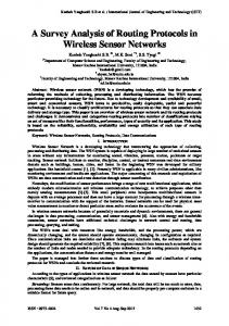
Routing has been carried out in sensor networks with the basis on conserving energy. Power efficiency is the most important design metric as it is an important design goal of any sensor network. Routing algorithms are also data centric and employs attribute based addressing strategies along with location awareness. These can be used with various clustering and hierarchical approaches to make an efficient routing algorithm for sensor networks. A robust and scalable stategy is required in designing a routing protocol which is also energy efficient with minimal control overhead. Different routing protocols in sensor networks can be divided into six categories based on their underlying architectural framework. These different categories are as follows (see Figure 1). • Attribute-based (Section 4.1) • Flat (Section 4.2) • Geographical (Section 4.3)

• Hierarchical (Section 4.4) • Multipath (Section 4.5) • QoS-based (Section 4.6)

Routing protocols in sensor networks

Attributebased

Flat

Geographical

Hierarchical

Multi-path

QoS-based

Directed Diffusion

GRAdient

SPEED

LEACH

M-MPR

SER

EAD

SAR

Rao et. al

PEGASIS

Ganesan et. al

Arrive

Youssef et. al

MCFA

Seada et. al

TEEN/APTEEN

ReInForM

Subramanian et. al

Al-Karaki et. al

Rumor

Figure 1: Categories of Sensor Routing Protocols Some prior work discussing the various sensor network routing protocols have been [3, 7, 8, 9]. We list the classifications of sensor network routing protocols mostly based on the type of deployment of these networks. This classification helps the advent of newer ideas with special focus on the application being serviced by the sensor network and hence develop efficient algorithms to facilitate better routing techniques in these networks.

4.1

Attribute-based protocols

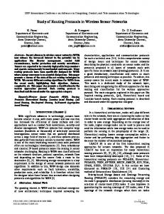
Attribute-based routing protocols in sensor networks concentrate on routing data packets based on the content of the packets and not device specific. Hence, these are also known as data centric routing approches. Since each node within the network is engaged in the routing mechanism, these nodes can take any decision and apply any routing rules to packets, i.e., either forward or drop the packets. In this class of routing algorithms, contents of the transmitted data are evaluated at each hop in the network. Directed Diffusion [10]: Directed diffusion is a data-centric approach which means all communications is for named data. It can be categorized under both attributed-based routing and flat routing protocols. Data generated by the application-aware sensor nodes is named using attribute-value pairs. A node requests data by sending interests for named data. A sensing task is disseminated via sequence of local interactions throughout the network as an interest for named data. Nodes diffusing the interest set up their own caches and gradients within the network to which the data delivery is carried out. During the data transmission, reinforcement and negative reinforcement techniques are used to converge to efficient distribution. Intermediate nodes fuse interests and aggregate, correlate or cache data. Energy-aware data-centric routing (EAD) [11]: This protocol proposes to build a virtual backbone which contains all the active sensors in the network to facilitate energy aware routing. Routing heuristic allows to build a broadcast tree rooted at a gateway to enable data-centric approach. The tree spans all sensors within the network and has a large number of leaves which save power by turning off their radios. The active sensors continue working as relays for traffic generated in the network. In data centric-routing, backbone senders are in charge of data processing and information dissemination throughout the network. At each individual sensor, the local raw data is initially combined/aggregated with

Event

Event

Source

Event

Source

Interests

Sink

Source

Gradients

Sink

Sink

Figure 2: Directed Diffusion [10] Algorithm 1 Pseudocode describing the Directed Diffusion algorithm Setup phase: 1. The base station broadcasts its set of interests 2. Do 3. ForEach network node N receiving an interest from node M 4. N forwards the received interest to its neighbors (other than M) 5. N sets up a gradient with M 6. EndFor 7. Until all gradients are set up 8. Check for loops in the paths and remove them Operating phase: 1. ForEach node 2. Colect sensor data. 3. Receive messages containing sensor data readings. 4. Aggregate, correlate or fuse data (if necessary) 5. If data maches an interest 6. Forward the data according to the gradient associated with the interest 7. EndIf 8. EndFor

data from other sensors located farther away from the sink. This aggregated data is then sent to a sensor closer to the sink or to the sink itself. EAD consists of two main components: the neighboring broadcast scheduling and the distributed competition among neighbors. These components ensure that the final tree has many leaves and sensors with relatively higher residual power also have a greater chance of being part of the virtual backbone. EAD basically makes certain the formation of a specially rooted broadcast tree designed for data centric routing. This protocol is suitable for applications requiring frequent queries and events. Constrained shortest-path energy-aware routing [12]: The distance from a source to a destination can be used as a metric for energy consumption and estimation of the propagation delay between them. It is shown that by changing the transmission power level and thereby changing the network topology graph, the algorithm can be optimized to ensure higher throughput and energy efficiency while maintaining lower end-to-end delay. The nodes are grouped into clusters with each cluster having a clusterhead or gateway node. Routing decisions are determined and maintained at the clusterhead. Such a centralized approach is more efficient than a distributed approach since it entails lesser control packet overhead maintainance. The network operates in two main cycles: data and routing. The data cycle consists of the nodes sending data to

the gateway nodes whereas during the routing cycle, the routing state of each node is determined by the clusterhead and the routing information sent to all the nodes accordingly. The constrained shortest path algorithm uses the distance between any two nodes to determine transmission power required to send packets from one to another. The transmission energy varies inversely with dn where d is the distance between the transmitter and receiver, n is a value based on the system and application in-use. The connectivity between nodes in a cluster can be maintained by this energy parameter making the network topology dynamic. If no constraints are enforced for the transmission energy, then each node uses its maximum energy to transmit directly to the destination. This is certainly not maintainable in the long run; therefore, a constraint has to be put in place. Rerouting is carried out by the clusterhead if (i) the sensors within the clusters are reorganized; (ii) the battery level of the active nodes falls under a certain threshold or (iii) there are some changes required in the energy model of the nodes. RUMOR [13]: Rumor allows the routing of queries to nodes that have observed an event of interest. As a result, retrieval of data is based on events and not on an addressing scheme. An event is an activity related to the phenomena being sensed (e.g. increased movement in an area being monitored). Events are assumed to be localized phenomena which occur in fixed regions of space. A query is issued by the sink node for one of two reasons, as an order to collect more data, or as a request for information. Once a query arrives at its destination, data is issued to the originator of the query. Depending on the amount of data (whether it is more or less) being issued to the originator of the query, shorter paths from the source to the sink are discovered. Any node may generate a query for a particular event. If it knows the route to the event, it transmits the query. Otherwise, the query is sent in a random direction, and this continues until the query reaches a node which has a route to the event. Each node has its neighbor list and an events table with forwarding information to all the events it knows. After a node witnesses an event, an agent may be created, which is a long-lived packet and travels around the network. Each agent contains an events table, including the routing information for all events it knows. Since an event happens in a zone, composed of several or many nodes, it is possible that multiple agents are created from the zone and moving in the network. When an agent travels in the network, its routing table is updated if there exist a shorter path to an event within the routing table of the node it is visiting. In a similar way, the routing table of the currently visited node is updated if its route to an event is more costly than the agents route. See Figure 3.

A

text

Event

Node with path to event

Event 1

Node

Query source = query path to event

Event 2

Node with path to event 2

Agent

Node with path to events 1 and 2

A

Node with path to event 1

Figure 3: Rumor [13] Rumor routing uses agents, which have a limited life determined by a TTL field; these agents create paths in the direction of any events they may come across. If an agent crosses a path to an event that it has not yet come across in the network, it creates a path that leads to both events. If flooding was to happen on a regular basis, network resources would be consumed quickly, thus Rumor

routing was created to be an alternative to flooding queries and events. When a query is generated, it is sent randomly through the network until it finds the event path instead of flooding it. When the query finds the event path, it is routed directly to the event. Only if the path cannot be found, it is flooded as a last resort.

4.2

Flat protocols

In flat sensor networks, there is a large number of nodes which collaborate together to sense the environment. These nodes are similar to each other in all respects and due to their sheer number they cannot be assigned specific global IDs. Routing protocols servicing such flat networks fall under this category of sensor networks. GRAdient Broadcast (GRAB) [14]: This protocol is designed for efficient data forwarding in large scale dense sensor networks where particular objects or events called stimuli are monitored by all the sensor nodes in the neighborhood. An earlier version of this work has been reported in [15]. These sensors pick up the same stimuli simultaneously but collectively elect a leader which creates a sensing report on behalf of the entire group. The election is carried out by the signal strength of the field created by the stimulus. All the nodes picking up the stimulus broadcast their respective signal strengths with a random delay to avoid collisions. Whenever a node hears this signal from another node, the node checks the strength of the signal and compares it with its own. If it is lower than the received signal, it stops otherwise it rebroadcasts its own signal strength. This helps in rolling the messages to the center of the stimuli (CoS) where ultimately the leader is chosen. This is the node with the largest signal strength and then it generates the report. This leader is named as the data source. On the other hand, each node always maintains a cost value, a metric representing the cost of sending data from the node to the destination sink. It is the job of the sink to build and maintain this cost field associated with each node, but the nodes also know their respective costs. Nodes located closer to the sink obviously have lesser cost values than ones which are located farther away. The main difference of GRAB from other protocols is that instead of the sender deciding the path for the data packet, it is the intermediate nodes who decide whether or not they should be forwarding the packet to the sink. This decision is taken by the receiver nodes simply by comparing their respective cost values with that of the sender and if it is lower, then they accept forwarding the packet. Due to this inherent mechanism, data will always be forwarded on the shorter path, i.e. the path of descending cost to the sink. However, some small issues come up if there are multiple paths to the destination. To solve some of these problems, the source also assigns a credit value along with the report it generates and sends out for transmission. With this credit value, a report may be sent out on a mesh of interleaved paths where none of the paths have a total cost greater than the cost of the source in addition to its credit. This simply makes use of the multiple paths if available and hence introduces a certain degree of robustness into the protocol. This degree of overhead and robustness is the “width” of the mesh, which is ultimately dependent on the credit of the report. This credit value also helps in controlling the robustness degree which may be useful for different scenarios and events occuring within the sensor network. No state information is required to be maintained at the individual nodes thereby eliminating overhead due to network complexity and path maintenance. Sequential Assignment Routing (SAR) [16, 17, 18]: This is the very first sensor routing algorithm to include QoS concepts. It is mainly a table-driven multipath approach towards routing and concentrates on energy efficiency and fault tolerance. Path selection is made by considering the energy resources of the nodes on the path along with the priority levels of each packet. The packet priority is calculated using an innovative technique. There is an energy cost and delay value associated with each link, which provides a resistance to packet flow. It is against this metric that a packet will have credits so that it achieves a certain priority in using these paths. A weighted QoS metric, which is the product of the additive QoS metric mentioned earlier and a certain weight coefficient, measures the QoS provided to each packet relative to the priority level of the packet [16]. The main objective of the SAR algorithm is to minimize this average weighted QoS metric. The SAR algorithm creates trees which have roots at the one-hop neighbors of the sink by taking the priority level of each packet, the QoS metric, and the energy resources for the nodes on each path. With

these trees, multiple paths are created and maintained from source to destination. When a path fails, the recovery procedure is carried out by forcing updates of the routing table between upstream and downstream nodes. Hence, there is always an available path for sending the packet and any path failure always leads to a local path restoration being carried, which mainly means updating the respective routing tables for the nodes. The major disadvantage of this protocol is that each node has to maintain entire routing tables of not only one path between a set of sources and destinations, but many available paths. This leads to greater overhead and memory requirements and also leads to more energy waste, specially in case of dense networks. Minimum Cost Forwarding Algorithm (MCFA) [15]: This paper presents a cost-field approach to minimum cost forwarding in sensor networks. The authors propose a “cost field”, which is defined as “the minimum cost from that node to the sink on the optimal path”. Since the direction of the routing is always known, the sensor node is not required to have unique ID or maintain a routing table, but rather each node maintains the minimum cost estimate from itself to the sink. Each sensor node broadcast the message to be forwarded to its neighbors. When the neighbor node receives the message, it verifies if it is on the minimum cost path towards the sink. If so, it broadcasts the message to its neighbors. This forwarding scheme continues until the message reaches to the sink.

4.3

Geographical routing

Geographical routing uses location devices to estimate the location of a node prior to forwarding the packets to the destination region. In wireless sensor networks, geographical forwarding (GF) is a widely used approach due to its low overhead and localized interactions. In GF, location information is exchanged with the neighbors and the neighbor closest to the destination is selected as a result of forwarding decisions. SPEED [19]: This is the stateless protocol for soft real time communication in sensor networks. Each node maintains information about all of its neighbors and uses a geographic forwarding technique to find the paths. The SPEED protocol tries to ensure a certain speed for each packet sent such that the application has an idea of the average end-to-end delay between the nodes. If the routing protocol makes the estimated speed of the packet available, the application can calculate this delay before-hand simply dividing the distance between the source and the sink by the estimated speed. The protocol also provides congestion avoidance mechanism when needed. The routing component, called the stateless geographic non-deterministic forwarding (SNFG), in SPEED uses four modules listed below to function effectively. 1. Beacon exchange: Similar to any other geographic routing algorithm, location information is updated periodically by nodes using specific beacon packets broadcast. Two other types of on-demand beacons in SPEED includes delay estimation and backpressure beacons. These are mainly used to quickly identify traffic changes in the network. 2. Delay estimation: This is carried out at each node by calculating the time elapsed since the acknowledgment receipt of the last data packet sent. By observing these delay values, the SNFG selects the best node conforming to the speed requirement of the application. 3. Neighborhood feedback loop: If no node with an appropriate delay value is obtained, this module is consulted for the relay ratio of the node. This ratio is simply the miss ratio of all the neighbors of the node, i.e. the nodes which were unable to provide the desired speed for the application. A random number between zero and one is generated and if the relay ratio is less than the random number generated, the packet is dropped. 4. Backpressure rerouting: This module helps to reduce congestion by sending messages to the source nodes such that alternate routes can be discovered.

Due to the stateless architecture of SPEED, it requires minimal memory and minimal MAC layer support. It also provides traffic load balancing and also enables QoS routing and congestion management in the sensor network applications. Geographic Routing with no Location Information [20]: This is a geographic routing algorithm which does not use any location information. The previous geographic protocols presented always assume the prescence of location identification techniques; however, this requirement cannot always hold. This scheme assigns virtual coordinates in such a scenario in which any other geographic routing protocols can be deployed without any location information. The protocol has three stages. The initial assumptions are gradually removed as the protocol proceed further. It is essential to point out that the virtual coordinates assigned to the nodes do not have to accurately match to the geography of the places, but they should reflect the underlying connectivity. The local connectivity information is used to set these coordinates. The three stages of the protocol are described below in detail. 1. Perimeter nodes know location: Initially, it is assumed that all perimeter nodes know their locations and the non-perimeter nodes are assigned virtual coordinates. The analogy used, which is borrowed from graph theoretic approaches, states that “each neighbor relation is represented by a force which pulls the neighbors together”. Thus, the force in the x- and y- direction is proportional to the difference in x- and y-coordinates of the nodes respectively. Iteratively, each node updates its virtual coordinates by calculating the average of x- and y-coordinates of the neighbor set of each node. As the number of iterations increase, the nodes tend to move towards the perimeter nodes closest to them and ultimately the algorithm converges to a steady state where the nodes are spread throughout the region. 2. Perimeter nodes are known: The perimeter nodes are aware that they are on the perimeter but unlike the first step, they do not know their location. Each perimeter node broadcasts a HELLO packet to the entire network to discover the hop-distance to every other perimeter node. These distance pairs are stored in a perimeter vector in which each perimeter node in turn broadcasts its perimeter vector to the entire network. As a result, every perimeter node becomes aware of its hop distance from other perimeter nodes. A triangulation algorithm is executed to enable the nodes to compute the coordinates of all the perimeter nodes in the network. The triangulation algorithm could fail under some conditions. As a part of the solution to this problem, two nodes are designated as bootstrap beacons. These nodes flood the network with HELLO messages. The perimeter nodes include these beacons in their triangulation algorithm to compute the coordinates of all the perimeter nodes. 3. No Location information: The nodes use the following criteria as stated in [20] to decide if they are perimeter nodes: if a node is the farthest away, among all its two-hop neighbors from the first bootstrap node, then the node decides that it is on the perimeter. Energy-efficient forwarding strategies for geographic routing in lossy wireless sensor networks [21]: The main aspect of geographic forwarding includes the greedy forwarding of message packets by a node usually to the neighbor located closest to the destination. This strategy works only under the following assumptions: (i) sufficiently dense network; (ii) accurate localization; and (iii) high link reliability irrespective of the distance within the physical radio ranges. It has been observed that even though the first two assumptions may hold for most types of systems, the final assumption regarding high reliable links will not be fully satisfied in a realistic scenarios. This is due the fact that wireless links are inherently unreliable in nature and are subject to various environmental conditions causing the weak links to drop a high number of packets. These packets are then retransmitted which leads to high energy consumption. In order to alleviate the problem, the neighbors are classified based on link reliability. Not only could some neighbor links be weaker than the others, their loss characteristics could also be different. Hence, a blacklisting/neighbor

selection scheme is devised to avoid the weak and unreliable links. The distance-hop energy trade-off performance metric is proposed for geographic forwarding. If the forwarding scheme aims at minimizing hops as in greedy forwarding, a significant energy consumption can occur due to transmitting and/or retransmitting the packets on long and possibly unreliable weak links. On the other hand, if smaller distances are covered across stronger links, more hops would be visited again causing increased energy usage. The optimal choice is generally in the transitional region between these two strategies. However, let us note that not too many links should be blacklisted since this would cause greater route disconnections and lower delivery rates. Geographic routing with limited information in sensor networks [22]: This protocol shows that even for instances where there is erroneous or limited location information due to faulty GPS, the order of routing delays is within a constant factor of straight-line greedy routing strategies. The limited information means that nodes only know the relative quadrant or zone where the destination node is situated. Nodes can be forwarded in the wrong direction if the GPS at nodes are faulty or biased even when the nodes have the correct destination coordinates. The four basic scenario models are discussed below. 1. Location errors (imprecise GPS): An angular error is introduced within greedy straight-line routing so that the packet is forwarded anywhere in the zone within the angle. 2. Limited destination information: It is assumed that the node has only a coarse estimate of the destination location such as the quadrant or half-plane information. 3. Small fraction of nodes with routing information: In this scenario, only a small fraction of nodes know about the destination quadrant. If a node which has no information about the destination has a packet to send, it simply selects a neighbor randomly to forward the packet. 4. Throughput-capacity networks: The packet is forwarded in the right direction but not in a straight line along the shortest path. It uses specific progressive routing strategies to selectively forward the packets towards the destination. This leads to spatial “hot spots” within the network as many paths may intersect due to sub-optimal selection of routes.

4.4

Hierarchical protocols

As the name suggests this class of routing techniques create a virtual hierarchy among the nodes of the sensor network. Such a hierarchy may be based on zones which comprise of divisions of the entire network area, node functionality or node location. Irregardless of the system creating the network hierarchy, the routing protocol must be designed to make maximum use of this hierarchical pattern. Low Energy Adaptive Clustering Hierarchy (LEACH) [23]: LEACH is based on a simple clustering mechanism by which energy can be conserved since clusterheads are selected for data transmission instead th other nodes in the network. By the received signal strengths, local clusterheads are selected to serve as the routers to the data sinks. Sensor node sends its data to the local clusterhead in turn transmitted to the nearest clusterhead on the way to the sink. Since the clusterheads are only responsible for bulk of the data transfer, the overhead is minimized; however, if the clusterheads are chosen beforehand and remain fixed throughout the network lifetime, they will easily die out, thereby ending the lifetime of the member nodes of the particular cluster as well. To solve this problem, LEACH performs a periodic randomized rotation of the clusterhead to enable all the nodes within the cluster to take on a collective responsibility in order not to drain the battery of a single node. The optimal number of clusterheads is considered 5 percent of the total number of nodes. LEACH also performs local data fusion and aggregation to compress the data received from each cluster. Sensor nodes are selected as clusterheads by the node choosing a random number between zero and one. The node is selected as a clusterhead for the current round if the number is less than the following threshold values:

à T (n) =

p if 1 − p ∗ (rmod p1 )

! n∈G

where p is the desired percentage of clusterheads, r is the current round and, G is the set of nodes which have not been clusterheads in the last p1 rounds. Once all the nodes are organized into clusters, the clusterhead will create a schedule for the nodes in its cluster which enables the radio components of each cluster node to be turned off for most of the time. Each node tranmsits its data to the clusterhead according to its schedule. On completion, the clusterhead aggregates and sends all the data to the sink. LEACH achieves a significant reduction in energy dissipation when compared with direct communication and other minimum energy routing protocols. Properties of LEACH includes (i) dynamic clustering to increase network lifetime; (ii) single-hop routing from node to clusterhead, hence saving energy; (iii) distributiveness; (iv) additional overhead due to clusterhead changes and calculations leading to energy inefficiency for dynamic clustering in large networks. Algorithm 2 Pseudo-code describing the operation of the LEACH protocol Setup Phase: In this phase clusters are created - clusterheads (CHs) are chosen 1. 2. 3. 3. 4. 5. 6. 7. 8. 9. 10. 11. 12. 13. 14.

ForEach (node N) N selects a random number r between 0 and 1 If (r < Threshold value) N becomes a CH N broadcasts a message advertising its CH status Else N becomes a regular node N listens to the advertising messages of the CHs N chooses the CH with the strongest signal as its cluster head N informs the selected CH and becomes a member of its cluster EndIf ForEach (clusterhead CH) CH creates a TDMA schedule for each node to transmit data CH communicates the TDMA schedule to each node in the cluster EndFor

Steady State Phase: 1. ForEach (regular node N) 2. N collects sensed data 3. N transmits the sensed data to the CH in the corresponding TDMA time slot 4. EndFor 5. ForEach (clusterhead CH) 6. CH receives data from the nodes of the cluster 7. CH aggregates the data 8. CH transmits the data to the base station 9. EndFor

Power-Efficient Gathering in Sensor Information Systems (PEGASIS) [24]: PEGASIS forms chains of the sensor nodes instead of forming multiple clusters as performed in LEACH protocol. Each node in the

chain can transmit and receive data from its neighbors. In the entire chain, one node is selected to transmit all the data received to the sink or base station. The chain construction follows a greedy approach. The problem of building a chain to minimize the total length is similar to the travelling salesman problem. The elected local leader in the chain waits for data from its closest neighbors. These neighbors first receive data from their own respective closest neighbors and aggregate the data before tranmsitting to the leader. The leader then sends the data received from its closest neighbors to the sink. Even though PEGASIS is similar to LEACH, it differs in the following ways. It uses multi-hop routing while only one node is selected to transmit to the base station. The reduction in overhead due to dynamic clustering as in LEACH leads to a performance gain of almost 100 to 300 percent in PEGASIS. This overhead is reduced when: (i) transmission distances of non-leader nodes are minimized; (ii) one transmission is made to the sink per round by aggregating all the data. This reduces local energy consumption but introduces a large delay for nodes farther away from the leader node of that chain. It also results in a single point of failure by the bottleneck created at the chain leader; (iii) the number of transmission among the nodes are reduced leading to overall energy efficiency. Threshold sensitive Energy Efficient sensor Network protocol (TEEN) [25]: TEEN protocol is designed to respond to sudden changes in the sensed attributes and uses a hierarchical model along with a data-centric mechanism. Clusters are formed in a hierarchical fashion at different levels with elected clusterheads serving as communication links between each other and the data sink. Initially, the clusters are formed after which each clusterhead broadcasts two threshold values to all the nodes. These are hard and soft thresholds for the sensed attributes. The hard threshold is the minimum possible value of an attribute based on which the sensor will be transmitting data to the sink. When the sensed value of the attribute is greater than this threshold, the data is sent to the clusterhead. This enables the nodes to transmit only relevant data. Once a value above the hard threshold is sensed, the node checks if the difference in the current and earlier values is greater than the soft threshold and if so, the new data is transmitted. Hard and soft threshold values can be adjusted per requirements allowing to control the packet transmissions. This protocol is suceeded by the AdaPtive Threshold sensitive Energy Efficient sensor network protocol (APTEEN) [26] which aims at capturing periodic data collections and respond to time-critical events. While the architecture remains the same as TEEN, APTEEN supports three types of data queries: (1) historical–to analyze and monitor past data values and take decisions based on these recorded values; (2) one-time–to take a snap view of the current network situation and visualize it at a particular time instant; (3) persistent–to monitor the network over a continuous time interval specially during an event taking place. Data aggregation–exact and approximate algorithms [27]: The aim is to develop better data aggregation and in-network data processing schemes for energy savings in sensor networks. These lead to lesser packet transmissions and reduce redundancy, thereby helping in increasing the network lifetime. The protocol employs a hierarchical model which uses data aggregation and and in-network processing at two different levels of the network hierarchy. A set of nodes, called the local aggregators (LA), are elected. These form a backbone routing architecture on which the first instance of data aggregation and routing is performed. From the set of LAs, another set of aggregators, called master Aggregators (MA), are selected to form the second level of nodes to carry out the second level of data aggregation. Since choosing the optimal set of MAs is an NP hard problem, a seperate integer linear program (ILP) is developed to identify the optimal MA set. The goal of maximizing network lifetime must be considered during the selection process of MAs. The time required to solve the ILP increases exponentially with the number of LAs. Three near optimal approximation algorithms, which serve dual purposes of selecting MAs and employing routing to the external traffic sink, are proposed. The differences from conventional data aggregation approaches are: (i) data aggregation is performed at optimal network points rather than at arbitrary points in other approaches. The selected points maximize the network lifetime; (ii) routing and data aggregation are carried out simultaneously with the proposed algorithms; (iii) there are no additional overheads due to dynamic clustering and

topologies. The architecture is simple and uses a fixed hierarchy of nodes with no additional complications.

4.5

Multipath routing

Multipath routing techniques compute multiple paths from source to destination to effectively route around failed nodes or invalid links. In single-path routing protocols, if a link fails, additional control packets have to be generated and broadcast to discover newer paths. Multipath routing avoids such pitfalls and there is always a secondary route ready in the event of a route failure. Meshed Multipath Routing (M-MPR) [28]: Two ways of effecting disjoint multipath routing (MPR) include (i) Disjoint (or split) MPR (D-MPR) with selective forwarding (SF) in which case each packet is sent along different disjoint routes and the decision of path selection is made by the source on packet-by-packet basis and (ii) D-MPR with packet replication (PR) (or limited flooding) where multiple copies of a data packet are transmitted simultaneously along multiple disjoint routes from a source to a destination. A meshed multipath is set up in three steps: (i) acquiring neighborhood information, (ii) route discovery, and (iii) route reply as described below. • Acquiring neighborhood information: Each active node broadcasts its ID, residual battery power, and location information to local neighbors. For each active neighbor i, a node maintains the following information in its database: IDi , locationi , residual poweri . Since the sensor nodes are considered stationary, period update on neighborhood status is not needed unless the node is entering to sleep mode or has just woken up. In this case, the nodes status is locally broadcast based on which of the neighborhood tables of nearby nodes are updated. • Route discovery: Each node attempts to form a meshed multipath based on the neighborhood database and location information of the controller node. So far, the intermediate node is allowed to accept multiple discovery packets. During source-to-destination route discovery process, at most two copies of a discovery packet are accepted by an intermediate node and the first arrived packet is forwarded to maximum two downstream neighbors nodes to ensure the reduction of the receiver complexity and power consumption of a node as can be seen from Figure 4. Maximum two forwarding node is chosen since this allows an alternate route with minimum possible extra control overhead.

S

D

Figure 4: M-MMPR: Source-to-destination meshed multipath [28] The route packet has the following fields: source ID, source location, intermediate node ID, next node ID1, next node ID2, destination ID, destination location, T T L where the IDs of forwarding nodes (next node IDi, i = 1, 2), intermediate node ID, and T T L values are updated at each intermediate stage. Each intermediate node maintains the following information in its routing database: previous node IDi, previous node IDn, next node ID1, next node ID2. Since several nodes is targeting the same destination, an intermediate node can have more than two “previous node” entries in its routing table

although there will be no more than two “next nodes” as can be seen from Figure 5. The list of “previous node” is bounded since the number of local neighbors are finite and no entry is created in the routing table for discovery packets coming from an upstream neighbor which is already listed in the list. If an intermediate node that has already forwarded a discovery packet receives another discovery packet, it updates the “previous node” list in its routing table and drops the packet.

c d

b y

x D

Figure 5: M-MPR: Meshed topology formed by many-sources-to-a-destination routes [28] Entry in the routing table at each node is maintained as a soft-state that is deleted after a time out unless a reply is received from a controller node. Since most sensor applications are data-centric, delay differences (jitter) between packet arrivals is not a big concern. No other resource reservation apart from storing and maintaining upstream and downstream nodes information is made during this phase; therefore, the route discovery phase can be considered as a topology construction process. • Route reply: Route reply message identifies the nodes comprised the meshed path. The controller node, upon receiving the discovery packets from a single source, selects the first two and sends a route reply following the original links by the route discovery packets in reverse direction with the following fields: source ID, source location, intermediate node ID, previous node ID1, previous node ID2. Each intermediate node changes the states of its corresponding entries from soft to permanent for the duration of its active participation, updates the fields of the reply packet other than the source information and forwards the reply packet to its upstream node. When forwarding the route reply message, the node does not require the knowledge of source information. In case of the discovery packets arriving to controller node from several sensor nodes, multicast reply is used. If an intermediate node is out of service or goes to sleep mode, the upstream nodes select necessary neighbors to sustain connectivity. Intermittent “link breakage” will not trigger reconfiguration of meshed multipath, instead it is handled using selective forwarding. In the constructed meshed topology, the number of downstream links is no more than two, whereas the number of upstream nodes can be more. As can be observed from Figure 5, node n has three upstream nodes: a, b, and c; and two downstream nodes: x and y. After the meshed multipath is constructed the information packet is forwarded from the source to the destination using either the packet replication (PR) or selective forwarding (SF) variants. The methods are explained below in a nutshell. • In PR, a source packet is copied from along all possible paths to its destination. To reduce power consumption due to transmission of multiple copies of the same packet, there is a provision of discarding the packets if a node receives more than one correct copy of the packet from one of the upstream nodes to be forwarded to the downstream node. • In the SF variant of M-MPR, if there are more than one downstream nodes are available at either the source or an intermediate node, the information packet is forwarded to only one of the nodes based on local conditions.

In addition to fault tolerance objective, selective forwarding approach along meshed multipath offers more efficiency than PR in terms of resource utilization and and congestion avoidance. The main difference between PR and SF is that in PR, the packet is intended for multiple neighbors in which each of them will receive and forward the packet whereas in SF, only one receiver will receive and forward the packet. Due to broadcast nature, M-MPR requires less transmission energy than D-MPR; MPR provides more flexibility in selective forwarding decisions than D-MPR, resulting in more successful packet delivery rate. Algorithm 3 Pseudocode description of the Meshed Multipath Routing algorithm Setup phase: 1. 2. 3. 4. 5. 6. 7. 8. 9. 10.

ForEach (node N) N broadcasts node information N listens to broadcast packets of neighboring nodes N adds the received information to the neighborhood database EndFor ForEach (node N) N forwards a route discovery packets to a maximum of 2 hops N listens to route discovery packets and sends route reply packets N listens to route reply packets and sets up the meshed multipaths. EndFor

Operating phase: 1. 2. 3. 4. 5. 6. 6. 7. 8.

ForEach (node N) Select forwarding technique T. If T is packet replication N forwards data to all possible paths to the destination ElseIf T is selective forwarding N chooses a path to destination based on some criteria N forwards the data on the selected path EndIf EndFor

Highly-resilient, energy-efficient multipath routing in wireless sensor networks [29]: Energyefficient multipath routing defines a set of localized algorithms to construct multiple paths from the source to the destination. These multiple paths may come in handy if one particular route fails during the network operation. Multipaths are constructed between nodes using two different approaches. The first is the original node disjoint paths where none of the paths created intersect with each other meaning that they are completely disjoint. This ensures that for k paths constructed, no k node failures can eliminate all the paths. The second technique defines the braided paths in which there are generally no completely disjoint paths, rather numerous partially disjoint alternative paths. Conventional approaches to energy-efficient and robust routing have resulted in periodic flooding of the network, which in turn lead to energy inefficiency. By constructing alternate paths initially, there may be no need for periodic flooding of the data packets. In the event of the primary path failure along with all the other alternate paths simulatenously, there is no other option left but flood the network to ensure that the data reaches the destination. However such a condition should not occur very frequently. The two mechanisms for identifying disjoint paths and braided paths are as follows: • Disjoint multipaths: These can be constructed by identifying a few alternate paths which are node

Source

Sink

Sink

Low-rate samples

Primary-path reinforcement

(a)

Source

(b)

Source

Sink

Source

Sink

B

P alternate-path reinforcement

negative reinforcement

A

P1

(c)

X

(d)

Q Source

Sink B P

A P1

(e)

Figure 6: Construction of localized disjoint paths. The diagram (a) presents the low-rate date sample. Primary path P and the alternate path negative reinforcement are shown in diagrams (b) and (c) respectively. The alternate path P1 and the idealized algorithm are given in diagrams (d) and (e) [29]

disjoint with the primary path. Here, initially the primary path is selected between the source and the sink. This is followed by selecting the first alternate path as the best-path which is node disjoint with the primary path. Other secondary paths are selected based on the first disjoint path and this process continues till the number of alternate paths reach the maximum specified limit. These disjoint paths are resilient, but generally energy inefficient. See Figure 6 [29]. • Braided multipaths: In this technique, the alternate paths created are not completely node disjoint from the primary path, rather have a few nodes in common. Selecting a braided path is similar to selecting disjoint paths; however, each node on the primary path receiving a reinforcement propagates it to its most preferred neighbors who in turn carry out the same operation. This ultimately leads to multiple alternate paths, some of which can be parts of the primary path and are not completely node disjoint. See Figure 7 [29]. In this system, two different modes are considered, isolated and patterned node failures. In the first case, each node has an individual probability of failure whereas in the second case, all nodes within a particular radius fail simultaneously. ReInForM [30]: The reliable information forwarding using multiple paths (ReInForM) protocol brings to the forefront issues relating to information aware data delivery in sensor networks. It may happen that

a(i)

a(i)

a(i-1)

a(i-1)

Source

Sink n(k+1)

n(k)

n(k-1)

n(k-2)

a(i-2)

a(i-3)

(a)

n(k-3)

n(k+1)

n(k)

n(k-1)

n(k-2)

n(k-3)

a(i-2) (b)

Figure 7: Braided multipaths. The diagrams (a) and (b) present idealized and localized braided multipaths [29]

essential data is sent along a lossy and unreliable route. Let us look at an example in which a sensor network senses temperature at some points in the forest. On a given day, a sensor may sense a temperature of 60◦ F at a particular point which is normal. On the other hand, at that very moment, another sensor placed some distance away may be sensing a temperature of 1000◦ F. This packet containing the abnormal temperature is the more important packet and should be sent to the sink by more reliable links to ensure delivery with the lowest latency. Basically, the proposed mechanisms support delivery of data at any desired reliability. However, with the increase in reliability, one expects an increase in the overhead required to transfer the packet. Multiple paths from source to destination are discovered while reliability is ensured by redundant copies of a packet. The desired reliability, the local channel error conditions, and the neighborhood information at each node determines the degree of redundancy needed. Another key feature is that data caching is not required at intermediate nodes, thereby saving memory. In multi-hop sensor networks where the source is located far away from the sink with high number of channel error occurences, a simple packet forwarding strategy may become unreliable. To improve the reliability, two solutions have been proposed: (i) no acknowledgements–sending data from source to sink along the shortest path with no acknowledgements. Multiple copies of the packet are sent along the same path to increase the probability of packet delivery; (ii) with acknowledgements–sink sends back an acknowledgment to the source after receiving the data packet. The simulation results show that the acknowledgement based scheme has similar overhead to the non-acknowledgment based scheme. Hence, the no acknowledgment scheme is used in the protocol description. ReInForM is based on the Dynamic Packet State (DPS) [31] approach used for data networks. The source uses local knowledge of the network such as channel error, hop count to sink, etc. and sends multiple copies of the data packets through multiple paths. With every hop, network conditions are recorded in the packet header and forwarded to the next node. Every intermediate node takes forwarding decisions based on this stored information. This strategy enables the forwarding node to route the packets according to local network conditions, but without maintaining the state information on its own. It also helps in making localized decisions on packet forwarding since network characteristics at an earlier point on the path may be much different than at the current point. This mechanism adapts to channel errors and topological deviations while maintaining a reasonable overhead.

4.6

QoS-based protocols

Routing is generally carried out based on metrics prominent among which are control packet overhead and energy efficiency. However, additional Quality of Service (QoS) parameters may also be considered to facilitate more efficient routing in sensor networks. Stream-Enabled Routing (SER) [32]: SER protocol allows sources to choose the routes based on the

instruction (or task) provided by the sinks. An instruction is a predefined identifier value. Therefore, only identifier is sent rather than the attribute list, resulting in memory conservation. It takes into account the available energy of the sensor nodes, QoS requirements of the instruction, memory limitation of nodes, and the localized effect of dense nodes. Sinks can give new instructions to the sources without establishing another path. SER uses four types of messages: (i) Scout message (S-message), (ii) Information message (I-message), (iii) Neighbor-neighbor message (N-message), and (iv) Update message (U-message). S-message is used during the source discovery to determine sources that will process the instruction (or task) specified in the S-message. Sources decide the type and level of the routes needed by the instruction. There are four types of routes, each with two levels (i.e., level-1 and level-2). The µ value is the radius of the level-2 routes. Stream is identified by both the type and the level of route. Each level-2 stream includes level-1 stream. In level-2, the size of the radius µ of the stream can be determined based on QoS specified in the instruction. Combination of types and levels creates different kinds of QoS for a stream. After streams are chosen, the source sends N-message to establish the streams back to the sink. The repairs of streams are accomplished via N- and S-messages. Once the streams are accomplished, data travels from sources to the sink through either level-1 or level-2 stream with I-message. The sink can update the instruction (or task) at the sources through either level-1 or level-2 stream using U-message. Both sources and sink can terminate the streams using U-message. SER has seven phases: 1. Source Discovery. A sink broadcasts an S-message to find routes from sink to source. S-message contains the following fields: T ID, N AP, LID, N H, AE. Table 1 represents the parameters used throughout the algorithm description. Table 1: SER protocol parameters T ID N AP LID NH AE LI MT IN S T LOC DSP NS DLID U LID SLID M ES FI CN H P ayload N IN S

Task ID Network Access Point (represents a unique sink) Local ID No. of Hops from the sink Average Energy of a route Length Indicator Message Type, (MT=0 (S-message); MT=1 (I-message); MT=2 (U-message); MT=3 (N-message) Instruction Targeted Location Downlink Sensor Problem Node Selected LID of downlink sensor node LID of uplink sensor node Selected ID Message Flow Indicator (message going uphill or downhill) Current No. of Hops Description New INS

Average energy of a node is given by the following formula: AE =

N Hi−1 × AEi−1 + Ei N Hi−1 + 1

The T ID field is further composed of LI, M T, IN S, and T LOC fields. When a sensor node receives an S-message, it determines if the instruction, (IN S), is intended for the node. If the IN S in the

S-message is not intended for the node, the node stores the fields of S-message in a connection-tree (C-tree). C-tree is a logical tree which represents possible connections through the node. It maintains the nodes neighbors that can participate in a routing back to sink. A sensor node in an established route knows the LID values of both uplink and downlink nodes Initially, DLID and U LID values are not set and DSP and N S values are set to OFF. Updated values of AE, N H, and LID fields of S-message is broadcast to the neighbors. If sensor node receive the same S-message from its neighbors, it dismisses it. The sources store S-message in a task-tree (T-tree). T-tree has x DLID values since source can select up to x LIDs to route I-message back to the sink based on QoS requirement. The max value of x is the number of neighbor nodes. Each DLID value corresponds to a DSP indicator. In the T-tree, the leaf nodes has no U LID and N S indicator since sources are destination of S-message. A source can receive x S−message since it has x neighbors. Route associated with the first received S-message is considered the shortest route. Sources select neighbor node to send I-message back to sink based on the QoS requirement of IN S. 2. Route Selection. Once the sources receive the S-message, they determine the QoS requirement of task in the S-message. There are four types of streams for communication between sources and sinks and each stream can either be level-1 or level-2: • Type 1: Time Critical But Not Data Critical • Type 2: Data Critical But Not Time Critical • Type 3: Not Time and Data Critical • Type 4: Not Time and Data Critical After the sources select the neighbor nodes, the sources broadcast an N-message to their neighbors indicating the level and size of the stream. N-message contains T ID, N AP, LID, SLID, and M ES fields. If stream is level-1, µ = 0 (width of the stream). At level-1, messages are routed back to the sink via hop-by-hop communication. Messages are sent to only one node. Level-2 stream contains level-1 stream which serves as a backbone in setting up level-2 stream. The value of µ is the number of hops away from the nodes in the level-1 stream. Messages can flow downhill to the sink or uphill to the sources by flooding through only the nodes that are part of the stream. I-message flows downhill from sources to sink by using N H value stored in each node in the C-tree. The nodes near to the sources have higher N H values. U-message flows uphill from sink to sources by using the negative of N H value. The nodes near to the sources have higher negative N H values. 3. Route Establishment. N-message is used by a sensor node to inform neighbors about its local information. The source sends an N-message to establish stream back to the sink. Sensor nodes that are not part of a stream delete all data associated with N-message from C-tree. If intermediate nodes between the sources and sinks have not received an N-message in response to S-message in a set time interval, the sensor node deletes the C-tree branch that is associated to S-message. After the N-message arrives to the sink, the minimum delay or maximum average energy stream is established. Sources can start sending I-messages to the sink. I-message contains T ID, F I, CN H, and P ayload fields. 4. I-message Transmission. The neighbor nodes can determine if they need to route the I-message by the T ID since each neighbor nodes maintain a C-tree. When a source broadcasts I-message, it sends CN H field with the value from T-tree. Intermediate nodes between sources and sink use C-tree. F I and CN H fields are only used when the stream is level-2. Each node only rebroadcasts once to avoid a node from broadcasting the same message over again. After an I-message is received, the sensor nodes turn OFF the receiver for some amount of time if the sleep mode operation is ON such that the node can avoid listening neighbors broadcasting the same I-message. C-tree indicates which instructions the sensor nodes need to route.

5. Route Reconnection. If a sensor node is low on energy or there is too much noise around when transmitting at level-1, it can broadcast an N-message by setting up reconnect message indicator. Once the neighbors receive N-message, they check their C-tree to decide if there are possible alternate routes. N-message will be broadcasted until the alternate route is found. Sudden death of route: If the stream suddenly terminates, sink cannot get the I-messages. The sink sends out a new S-message with higher QoS requirement version of the same instruction (higher QoS IN S value). New streams can be found to avoid broken paths. Multiple streams of level-2 can be setup between source and sink to improve robustness of I-message routing. 6. Instruction Update. U-message allows sink to update its instruction to the sources. The U-message from the sink to the sources flow uphill while it flows downhill from sources to the sink when streams are level-2. U-message contains T ID, F I, CN H, and N IN S fields. 7. Task Termination. A task at the sources are terminated in two ways: (a) Sources have finished the task associated with the instruction given by sink. U-message with the task completed instruction indicator is broadcast by sources. (b) Sink decides to terminate the instruction. U-message with the task termination instruction indicator is set by the sink. The streams are torn down by removing C-tree braches at the intermediate nodes and T-tree at the sources. Algorithm for Robust Routing in Volatile Environments (ARRIVE) [33]: This is a probabilistic algorithm and makes packet forwarding decisions based on localized information and it has a tree-like topology rooted at the sink of the network. The forward approach is employed to achieve end-to-end reliability. The packet loss is avoided by sending multiple packets of the single event. Basically, the three sources of packet loss expected are (i) isolated link, (ii) patterned node failures, and (iii) malicious or misbehaving nodes. The following presents the terminology of the algorithm: • Event: Identified by [SourceID, EventID] • Level: Each node has unique level indicating distance from source to sink (in terms of hops) • Parents: Nodes one level closer to the sink • Neighbors: Nodes on the same level and be able hear each other • Push: Push packet to one of the neighbors • Forward: Forward packet to one of the parents • Forwarding Probability: Included in the packet header and used to probabilistically select whether to push or forward • Reputation History: Each node keeps this information for each of its parents and neighbors • Convergence: Prevents multiple packets of the same event being sent to same source of failure ARRIVE achieves diversity in paths in two ways: (i) upon receiving a packet, the next hop is selected probabilistically based on link reliability and node reputation and (ii) when more than two or more packets of the same event are processed, these packets are ensured to follow different outgoing links. Each keeps the following information: level, neighbors list, parents list, reputation history of neighbors and parents, and convergence history of specific events.

Waiting for packet

No

packet received passively process packet

No

is packet for me?

Yes Yes

Neighbor

check threshold conditions

where to send packet?

check threshold conditions

Parent

check threshold conditions

send packet

Figure 8: Overview of Arrive protocol [33]

Several assumptions are made about the network and the algorithm. The network, which is almost considered a static network, is assumed to be dense enough for sufficient multiplicity of paths to exist between sources and sink for the algorithm to perform well. Sensors used are considered to have a low per-node cost. Routes used by the packets are unlikely to be optimal due to the probabilistic nature of the algorithm. Messages flow only from nodes to one and only sink. The bread first search rooted at sink is used to initialize level, parents, neighbors state information at each node. When a node hears a packets, it checks to see if the packet is addressed for it. If so, threshold processing takes place. Nodes are filtered by their reputation and convergence history of the neighbors and parents. A decision needs to be made to either to choose to forward the packet to a parent or push it to one of its neighbors with the probability value found in the packet header. This is randomly determined by the forwarding probability function P r(f ). Each node is weighed by their reputation. The destination is randomly selected from the rest of the nodes (since bad reputation nodes are eliminated). If the the packet is forwarded to one of the parents, P r(f ) is not changed; however, its value is increased.

5

Conclusions

In this chapter, we have discussed various routing protocols in sensor networks. The common goals of designing a routing algorithm is not only to reduce control packet overhead, maximize throughput, minimize the end-to-end delay, but also to take into consideration the energy consumption, especially in a sensor

Classification Attribute-based Attribute-based Attribute-based Attribute-based Hierarchical Hierarchical Hierarchical Hierarchical Hierarchical Multipath Multipath Multipath Geographical Geographical Geographical Geographical QoS QoS Flat Flat Flat

Protocol

Directed Diffusion EAD RUMOR Youssef et. al LEACH PEGASIS TEEN APTEEN Al-Karaki et. al M-MPR Ganesan et. al ReInForM SPEED Seada et al Subramanian et al Rao et. al SER ARRIVE SAR GRAdient MCFA

Restricted Virtual backbone Very restricted Cluster based Fixed base station Fixed base station Fixed base station Fixed base station No No No Limited No No No Yes No No No No No

Mobility

Power usage Limited Limited – Low Highest Highest Highest Highest – – High – – High – – – – – High Low

Negotiation based Yes No No No No No No No Yes No No No No – – No Yes Yes Yes No No

Table 2: Comparison of sensor network routing protocols Data Aggregation Yes Yes Yes Yes Yes No Yes Yes Yes No No Yes No Yes No – No Yes Yes No No

Restricted Restricted High Limited High High High High High Restricted High Restricted Restricted Restricted Restricted High Restricted Restricted Restricted High High

Scalability

network comprised of nodes which are considered light-weight with limited memory and battery power. We have divided the sensor routing protocols into six categories: i) attribute-based, ii) flat, iii) geographical, iv) hierarchical, v) multipath, and vi) QoS-based. We have then compared the protocols belonging to the same category based on various characteristics.

6

Questions 1. List the characteristics of Directed Diffusion protocol which makes it considered both flat and attribute based sensor routing protocol. 2. For which type of sensor applications is the EAD protocol most suited? Detail some of the factors by which EAD helps in providing better services to these applications. 3. On what basis are the local clusterheads selected in the LEACH protocol? Describe the clusterhead selection procedure in detail. Why are clusterheads not selected at the initial network deployment time itself? 4. How do PEGASIS and LEACH protocols differ? 5. In the ReInForM protocol, determine the reasons why the No ACK scheme has a similar control packet overhead to the ACK scheme, since at first glance it would logically seem that the scheme without the ACK packets would result in much less control overhead. 6. The SPEED protocol is characterized by minimal memory requirements. What are the probable reasons for such a characteristic? 7. ARRIVE protocol use a tree based routing approach. Discuss various advantages derived by using such a routing scheme.

References [1] D. E. Culler, D. Estrin, M. B. Srivastava, Guest editors’ introduction: Overview of sensor networks, IEEE Computer 37 (8) (2004) 41–49. [2] G. J. Pottie, W. J. Kaiser, Wireless integrated network sensors, Communications of ACM 43 (5) (2000) 51–58. [3] I. F. Akyildiz, W. Su, Y. Sankarasubramaniam, E. Cayirci, Wireless sensor networks: a survey, Computer Networks 38 (4) (2002) 393–422. [4] W. Ye, J. S. Heidemann, D. Estrin, Medium access control with coordinated adaptive sleeping for wireless sensor networks, IEEE/ACM Transactions on Networking 12 (3) (2004) 493–506. [5] V. Rajendran, K. Obraczka, J. Garcia-Luna-Aceves, Energy-efficient collision-free medium access control for wireless sensor networks, in: Proceedings of SenSys, 2003, pp. 181–192. [6] D. Estrin, R. Govindan, J. S. Heidemann, S. Kumar, Next century challenges: Scalable coordination in sensor networks, in: Proceedings of MOBICOM, 1999, pp. 263–270.

[7] S. Tilak, N. B. Abu-Ghazaleh, W. R. Heinzelman, A taxonomy of wireless micro-sensor network models, ACM Mobile Computing and Communications Review 6 (2) (2002) 28–36. [8] J. N. Al-Karaki, A. E. Kamal, Routing techniques in sensor networks: A survey, IEEE Communications 11 (6) (2004) 6–28. [9] K. Akkaya, M. Younis, A survey on routing protocols for wireless sensor networks, Ad Hoc Networks Journal 3 (2005) 325–349. [10] C. Intanagonwiwat, R. Govindan, D. Estrin, Directed diffusion: a scalable and robust communication paradigm for sensor networks., in: Proceedings of MOBICOM, 2000, pp. 56–67. [11] A. Boukerche, X. Cheng, J. Linus, Energy-aware data-centric routing in microsensor networks, in: MSWIM ’03: Proceedings of the 6th ACM international workshop on Modeling analysis and simulation of wireless and mobile systems, 2003, pp. 42–49. [12] M. A. Youssef, M. F. Younis, K. Arisha, A constrained shortest-path energy-aware routing algorithm for wireless sensor networks., in: Proceedings of WCNC, 2002, pp. 794–799. [13] D. Braginsky, D. Estrin, Rumor routing algorithm for sensor networks, in: Proceedings of WSNA, 2002, pp. 22–31. [14] F. Ye, G. Zhong, S. Lu, L. Zhang, Gradient broadcast: A robust data delivery protocol for large scale sensor networks, Wireless Networks 11 (3) (2005) 285–298. [15] F. Ye, A. Chen, S. Liu, L. Zhang, A scalable solution to minimum cost forwarding in large sensor networks, in: Proceedings of the tenth International Conference on Computer Communications and Networks (ICCCN), 2001, pp. 304–309. [16] K. Sohrabi, J. Gao, V. Ailawadhi, G. J. Pottie, Protocols for self-organization of a wireless sensor networks, IEEE Personal Communications Magazine 7 (5) (2000) 16–27. [17] K. Sohrabi, On low power wireless sensor networks, Ph.D. thesis, Electrical and Computer Engineering Department, UCLA (June 2000). [18] J. L. Gao, Energy efficient routing for wireless sensor networks, Ph.D. thesis, Electrical and Computer Engineering Department, UCLA (June 2000). [19] T. He, J. A. Stankovic, C. Lu, T. F. Abdelzaher, SPEED: A stateless protocol for real-time communication in sensor networks., in: Proceedings of ICDCS, 2003, pp. 46–58. [20] A. Rao, C. Papadimitriou, S. Shenker, I. Stoica, Geographic routing without location information, in: Proceedings of MOBICOM, 2003, pp. 96–108. [21] K. Seada, M. Zuniga, A. Helmy, B. Krishnamachari, Energy-efficient forwarding strategies for geographic routing in lossy wireless sensor networks., in: Proceedings of SenSys, 2004, pp. 108–121. [22] S. Subramanian, S. Shakkottai, Geographic routing with limited information in sensor networks., in: Proceedings of IPSN, 2005, pp. 269–276. [23] W. R. Heinzelman, A. Chandrakasan, H. Balakrishnan, Energy-efficient communication protocol for wireless microsensor networks, in: Proceedings of HICSS, 2000. [24] S. Lindsey, C. Raghavendra, PEGASIS: Power-efficient gathering in sensor information systems., in: Proceedings of IEEE Aerospace Conference, 2002, pp. 1125–1130. [25] A. Manjeshwar, D. P. Agrawal, TEEN: A routing protocol for enhanced efficiency in wireless sensor networks, in: Proceedings of IPDPS, 2001, pp. 2009–2015.

[26] A. Manjeshwar, D. P. Agrawal, APTEEN: A hybrid protocol for efficient routing and comprehensive information retrieval in wireless sensor networks, in: Proceedings of IPDPS, 2002, pp. 195–202. [27] J. N. Al-Karaki, R. Ul-Mustafa, A. E. Kamal, Data aggregation in wireless sensor networks - exact and approximate algorithms, in: Proceedings of IEEE Workshop on High Performance Switching and Routing (HPSR), 2004, pp. 241–245. [28] S. De, C. Qiao, H. Wu, Meshed multipath routing with selective forwarding: an efficient strategy in wireless sensor networks, Computer Networks 43 (4) (2003) 481–497. [29] D. Ganesan, R. Govindan, S. Shenker, D. Estrin, Highly-resilient, energy-efficient multipath routing in wireless sensor networks, ACM Mobile Computing Communication Review 5 (4) (2001) 10–24. [30] B. Deb, S. Bhatnagar, B. Nath, ReInForM: Reliable information forwarding using multiple paths in sensor networks., in: Proceedings of LCN, 2003, pp. 406–415. [31] I. Stoica, S. Shenker, H. Zhang, Stateless fair queueing: Achieving approximately fair bandwidth allocations in high speed networks., in: Proceedings of SIGCOMM, 1998, pp. 118–130. [32] W. Su, I. F. Akyildiz, A Stream Enabled Routing (SER) Protocol for Sensor Networks, in: Proceedings of Med-hoc-Net, 2002. [33] C. Karlof, Y. Li, J. Polastre, ARRIVE: Algorithm for robust routing in volatile environments, Tech. rep., Technical Report UCB/CSD-03-1233, Computer Science Division, UC Berkley (May 2003).