Geosci. Model Dev., 7, 1183–1195, 2014 www.geosci-model-dev.net/7/1183/2014/ doi:10.5194/gmd-7-1183-2014 © Author(s) 2014. CC Attribution 3.0 License.
A technique for generating consistent ice sheet initial conditions for coupled ice sheet/climate models J. G. Fyke1 , W. J. Sacks2 , and W. H. Lipscomb1 1 Group
T-3, Los Alamos National Laboratory, Los Alamos, New Mexico, USA Center for Atmospheric Research, Boulder, Colorado, USA
2 National
Correspondence to: J. G. Fyke (
[email protected]) Received: 19 March 2013 – Published in Geosci. Model Dev. Discuss.: 15 April 2013 Revised: 7 April 2014 – Accepted: 23 April 2014 – Published: 23 June 2014
Abstract. A transient technique for generating ice sheet preindustrial initial conditions for long-term coupled ice sheet/climate model simulations is developed and demonstrated over the Greenland ice sheet using the Community Earth System Model (CESM). End-member paleoclimate simulations of the last glacial maximum, mid-Holocene optimum and the preindustrial are combined using weighting provided by ice core data time series to derive continuous energy-balance-model-derived surface mass balance and surface temperature fields, which are subsequently used to force a long transient ice sheet model simulation of the last glacial cycle, ending at the preindustrial. The procedure accounts for the evolution of climate through the last glacial period and converges to a simulated preindustrial ice sheet that is geometrically and thermodynamically consistent with the preindustrial CESM state, yet contains a transient memory of past climate. The preindustrial state generated using this technique notably improves upon the standard equilibrium spinup technique, relative to observations and other model studies, although in the demonstration we present here, large biases remain due primarily to climate model forcing biases. Ultimately, the method we describe provides a clear template for generating initial conditions for ice sheets within a fully coupled climate model framework that allows for the effects of past climate history to be self-consistently included in long-term simulations of the fully coupled ice sheet/climate system.
1
Introduction
Ice sheets play an important role in regulating critical aspects of the climate system such as sea level rise (Foster and Rohling, 2013), atmospheric circulation (Ridley et al., 2005) and ocean circulation (Weaver et al., 2003). Ice sheets can be considered coupled components of the climate system for several reasons. Ice sheet geometry is closely related to climate via the surface mass balance (SMB) and surface temperature (Cuffey and Paterson, 2010): SMB defines where ice accumulates or melts and thus helps determines ice sheet geometry, while advection of surface temperature into ice sheets regulates the internal ice temperature distribution and consequently ice rheology and basal sliding. Conversely, ice sheet presence and evolution is a fundamental control on regional to hemispheric circulation patterns (e.g., Manabe and Broccoli, 1985), oceanic freshwater fluxes (e.g., Broecker, 1994) and regional climate behavior (e.g., Langen et al., 2012). Coupled ice sheet/climate models are potentially powerful tools for understanding the behavior of ice sheets (Hanna et al., 2013) because they are able to simulate important feedbacks between ice sheets and climate and calculate the SMB using in-line energy balance calculations. Thus, an increasing number of fully coupled ice sheet/climate models are in active development and have recently been used to perform a wide range of experiments (e.g., Vizcaíno et al., 2010; Fyke et al., 2011; Gregory et al., 2012; Lipscomb et al., 2013). An important aspect of coupled ice sheet/climate simulations is the generation of consistent initial coupled ice sheet/climate conditions. In coupled climate models, including those with integrated ice sheets, full self-consistency
Published by Copernicus Publications on behalf of the European Geosciences Union.
1184 between all components of the climate model is required before prognostic experiments can proceed. In traditional non-ice-sheet-enabled models, this consistency typically is acquired through spin-up to a stable equilibrium, with all coupling between components enabled. Ice sheets excluded, the slowest component of coupled models to equilibrate is usually the deep ocean, which reaches steady state after ∼ 103 years; this deep-ocean spin-up time ultimately determines the coupled model spin-up simulation length. In typical preindustrial coupled climate model spin-up exercises, the primary goal is to obtain a coupled model state in which all the physical and biogeochemical components (including the deep ocean) are in equilibrium with each other and with recent Holocene climate forcings (insolation, radiative gases, etc.) at the year 1850. Inclusion of ice sheets in coupled models complicates this traditional ocean-limited preindustrial spin-up approach, for the basic reason that ice sheets reach quasi-equilibrium on average deep ice residence and lithospheric relaxation timescales, i.e., ∼ 104 –105 years (i.e., 1–2 orders of magnitude slower than the ocean). This long equilibration time means that the present-day Greenland and Antarctic ice sheets (GrIS/AIS) are not in full equilibrium with preindustrial (i.e., recent Holocene) climate. Rather, they contain a remnant thermal and dynamic memory of past glacial periods that is reflected in present-day ice sheet conditions and potentially in long-term future ice sheet projections. Computationally efficient stand-alone ice sheet model simulations forced with simple and highly parameterized climate representations driven by various paleoclimate time series are able to simulate the 104 –105 years necessary to capture this memory (e.g., Huybrechts, 2002; Applegate et al., 2012). However, an analogous synchronous fully coupled spin-up with a computationally expensive fully coupled ice sheet/climate model is simply not possible. Several approaches have been introduced to circumvent this computational barrier to generating preindustrial coupled ice sheet/climate initial conditions. However, each method displays significant shortcomings: – A computationally cheaper climate parameterization can be used to force an ice sheet model through one or more glacial periods. At some point, the resulting ice sheet could be inserted into the climate model (Vizcaíno et al., 2010). Shortcoming: this approach results in an artificial discontinuity in the ice dynamic response due to a step-function change in climate forcing that potentially affects future simulations. – A positive-degree-day (PDD)-based SMB model could be used for past climates, with anomalies of modelsimulated preindustrial temperature/precipitation conditions calculated using paleoclimate time series (Quiquet et al., 2013). Shortcoming: an analogous approach to scaling inputs to the SMB model is not feasible for more Geosci. Model Dev., 7, 1183–1195, 2014
J. G. Fyke et al.: Ice sheet spin-up for coupled models physically consistent energy-balance-based SMB models. Also, if a PDD model is used during spin-up, a discontinuity will occur at the transition to the more consistent energy balance surface calculations within the coupled climate model framework. – Asynchronous coupling could be used to accelerate the ice sheet and orbital forcings, relative to the rest of the climate. Shortcoming: abyssal-ocean- and ice-sheetrelated limits to asynchronicity (Calov et al., 2009) still necessitate an extremely long climate simulation of 10 kyr or more to cover the entire last glacial cycle. – The ice sheet/climate model could be spun up under constant preindustrial forcing (Fyke et al., 2011). Shortcoming: while this approach may be valid for decadalto-century-scale simulations (Seroussi et al., 2013), neglecting past climate history on preindustrial ice sheet conditions will affect the longer century-to-millennialscale dynamic response of the ice sheets in coupled model simulations. These issues point to a requirement for an alternate method for generating spun-up ice sheets that (a) is driven by uncorrected conditions generated with integrated coupled climate model energy balance calculations; (b) has an internal memory of the past glacial climate state (specifically as represented by bias-uncorrected paleoclimate climate simulations) and (c) is self-consistent with the state of the climate-modelsimulated preindustrial climate. These constraints must be satisfied so that the resulting ice sheet state can be “inserted” into a fully coupled framework as part of the suite of selfconsistent component model initial conditions. In this study we describe and demonstrate one method for achieving this goal. A summary of this paper is as follows: we first detail the SMB and ice sheet models, the procedure for generating transient SMB forcing for the last glacial period and how this forcing drives an ice sheet model. We then demonstrate the ability of this method to simulate a transiently spun-up preindustrial ice sheet that exhibits dynamic and thermodynamic memory of past climate, yet is consistent with a simulated preindustrial climate model state and shows notable improvement relative to an equivalent equilibrium spin-up, when compared to relevant observations. Finally, we discuss potential future ice sheet and climate model developments that could further improve the transiently spun-up preindustrial ice sheet state (but which are outside the scope of the methods description presented here) and briefly contrast spin-up of ice sheet models with inversion-based initialization methods in the context of coupled ice sheet/climate modeling.
www.geosci-model-dev.net/7/1183/2014/
J. G. Fyke et al.: Ice sheet spin-up for coupled models 2 2.1
Models and methodology
1185 2.2
End-member climate SMB and temperature generation
Models
To develop a preindustrial ice sheet state that is compatible for use in a fully coupled modeling framework, we use a toolchain of models within the Community Earth System Model (CESM) framework. These include the fully coupled climate model CCSM4 (Gent et al., 2011), the stand-alone Community Land Model Version 4 (CLM; Oleson et al., 2010) and the Community Ice Sheet Model (CISM; Lipscomb et al., 2013) within CESM1.1. We point the reader to the above references for detailed technical descriptions of CCSM4, CLM4 and CISM. Briefly, we summarize here that CISM is a shallow-ice-approximation thermomechanical ice sheet model on a 5 km resolution GrIS grid. It includes a simple parameterization of basal sliding that depends on the presence of basal ice at the pressure melting point and a simple calving prescription in which all ice at floatation is instantaneously removed. SMB and surface temperature calculations over the GrIS are calculated using a full energy-balance-based SMB model at multiple vertical levels in CLM, the elevations of which are explicitly set to cover the full potential range of GrIS elevations. Importantly, SMB and surface temperatures are calculated at each time step in a full (x, y, z) matrix that includes locations where the GrIS surface does not exist. This feature is critical in the context of the ice sheet spin-up procedure described below, because it allows SMB and surface temperature values to be easily and directly interpolated to the evolving GrIS ice topography. This avoids complexities related to generating SMB lapse rates (Helsen et al., 2012) since it allows vertically interpolated climate-model-derived SMB values to be used directly during the ice sheet model simulation. The ice sheet spin-up technique described here using CCSM4, CLM and CISM simulations can be briefly stated as follows: the coupled CCSM4 climate model was used to simulate last glacial maximum (LGM), mid-Holocene optimum (MHO) and preindustrial climate states. Using output from these simulations, a corresponding set of CLM land surface model simulations were carried out to generate SMB and surface temperatures over Greenland for LGM, MHO and preindustrial climates. Composite SMB and surface temperatures at times between these “end-member” climate states were then calculated using weighting based on the North Greenland Ice Core Project (NGRIP) ice core δO18 record (Wolff et al., 2010). This series of forcing fields is finally downscaled via interpolation to the ice sheet model topography to drive a long CISM ice sheet model simulation. This process is described in more detail below and detailed graphically in Fig. 1.
Previously, Brady et al. (2013) generated fully coupled equilibrium climate states for the LGM and MHO using the CCSM4. This same model configuration was also integrated to equilibrium under preindustrial conditions (Landrum et al., 2012). These “simulations of opportunity” provided us with end-member climate states to use in testing our spin-up procedure. Unlike more recent versions of the CESM, the version of CLM within these CCSM4 simulations did not include in-line SMB calculations. However, included in the output of each of these large-scale simulations were the necessary atmospheric fields required to drive an updated version of CLM, which includes calculations for generating in-line SMB and surface temperature values at multiple elevation levels over Greenland. We thus used the final 30 years of output from the previously performed coupled climate model simulations of the LGM, MHO and preindustrial periods as looped input forcing for three corresponding CLM4 simulations, which were integrated for 200 years each to equilibrium and from which the final 30 years of equilibrium LGM, MHO and preindustrial SMB and surface temperature matrices were obtained at multiple vertical levels on the coarse CLM4 grid. These 30 year equilibrium SMB and surface temperature climatologies formed the basis from which the continuous forcing for the long transient ice sheet model spin was generated (Sect. 2.3). The downscaled end-member LGM, MHO and preindustrial SMB and surface temperature fields based on these climatologies are shown in Figs. 2 and 3. To ensure a sufficient spin-up length, the simulation was initialized at the end of the last interglacial (LIG). However, an appropriate fully coupled CESM LIG simulation was not available. We thus assumed the MHO to be the best approximation for the LIG and copied this forcing state for use as an idealized initial end-member LIG SMB forcing. The bias in ice sheet evolution resulting from using MHO forcing as a proxy for LIG climate conditions had little effect on the final preindustrial ice sheet state (which was the primary target of the simulation) since the memory of this forcing was swept from the system during the cold glacial period (Sect. 3). Full 30-year climatologies of SMB and surface temperature were used to ensure that both the mean climatology and any non-zero impacts on ice sheet evolution due to interannual SMB variability about the mean (Pritchard et al., 2008) were properly captured. 2.3
Continuous ice sheet model boundary condition generation
In order to provide continuous forcing for a 122 kyr ice sheet model spin-up simulation ending at the preindustrial, it was necessary to create SMB and surface temperature matrices between the end-member climate states. This www.geosci-model-dev.net/7/1183/2014/
Geosci. Model Dev., 7, 1183–1195, 2014
Discussion Paper
1186
J. G. Fyke et al.: Ice sheet spin-up for coupled models
MHO CCSM simulation
Preindustrial CCSM simulation
LGM CLM simulation
MHO CLM simulation
Preindustrial CLM simulation
|
Passed: end-member SMB/temperature forcing fields
Discussion Paper
Passed: atmospheric forcing fields
|
LGM CCSM simulation
Transient ice sheet spin-up simulation Fig. 1. Work flow for the procedure described in this study. Atmospheric output from global model simu-
Discussion Paper
End-member forcing fields interpolated using NGRIP weighting
|
lations is used to drive land-surface modelAtmospheric simulations. These simulations generate surface mass balance Figure 1. Work flow for the procedure described in this study. output from global model simulations is used to drive land-surface necessarygenerate to force the sheet model (after ice core data-weighted interpolation model simulations. Thesefields simulations theicesurface masssimulation balance fields necessary to force the ice sheetbemodel simulation (after ice tween bounding end-member SMB and temperature fields, and interpolation to the ice sheet geometry). core data-weighted interpolation between bounding end-member SMB and temperature fields and interpolation to the ice sheet geometry). Blue boxes: End-member simulations; red boxes: fields passed from one simulation to the next; grey Blue boxes: end-member arrow: simulations; fields passed simulation tofor thethenext; arrow: final ice sheet simulation. Note final ice red sheetboxes: simulation. Note use offrom MHOone climate as a proxy LIG grey (diagonal arrow). use of MHO climate as a proxy for the LIG (diagonal arrow). Discussion Paper |
was done using a technique adopted and modified from (Figs. 2 and 3): stand-alone ice sheet model spin-up approaches. First, rep- 28 δ 18 OEM+1 − δ 18 OCC resentative LGM, MHO(/LIG) and preindustrial δO18 val, (1) wt−1 = 18 δ OEM+1 − δ 18 OEM−1 ues were calculated by averaging the 600 years of NGRIP values bounding each time period from the NGRIP δO18 wt+1 = 1 − wt−1 , (2) record (Wolff et al., 2010) (for the preindustrial climate, yr=1:30 yr=1:30 SMB(x, y, z)CC = [SMB(x, y, z)EM−1 wt−1 ] NGRIP values corresponding to the interval 1250–1850 were yr=1:30 used). The 600-year averaging avoided aliasing of LGM, + [SMB(x, y, z)EM+1 wt+1 ], (3) MHO and preindustrial end-member climate NGRIP valyr=1:30 yr=1:30 T (x, y, z)CC = [T (x, y, z)EM−1 wt−1 ] ues due to centennial-scale variability in the NGRIP record. 18 The δO record was then thresholded slightly to account yr=1:30 + [T (x, y, z)EM+1 wt+1 ], (4) for the fact that time periods represented by the climate model end-member simulations did not fall exactly on maxiwhere EM−1 and EM+1 represent bounding end-member climum/minimum MHO/LGM NGRIP values. This avoided armates for a particular mid-run climate period CC and CC intificial extrapolation of SMB values beyond the cold/warm creases by 1 for every 600-year period (for example, for a LGM/MHO cases, which would have potentially introduced period CC in middle of the last glacial period EM−1 = LIG non-realistic extrapolated SMB values such as negative SMB and EM+1 = LGM). The interpolated 30-year SMB/surface at the summit during the LGM and too-high accumulation temperature climatology was then looped 20 times to produring the LIG/MHO. The practical impact of this threshvide the forcing for the 600-year CC period, with the reolding was to set SMB values of cold pre-LGM glacial perisulting daisy chain of looped climatologies providing the ods between interstadials to slightly higher model-simulated time-continuous forcing for the long continuous stand-alone LGM values, despite suggestions from the isotopic record CISM ice sheet simulation (after downscaling from the mathat these periods were actually slightly more extreme. trix of SMB and surface temperature values to the GrIS toThe resulting thresholded NGRIP δO18 record was then pography). Use of 600-year constant-climate climatologies, used to guide the time interpolation between the end-member instead of continuously interpolated SMB and temperature SMB and surface temperature matrices for every time step fields, was driven primarily by technical challenges encounand (x, y, z) location between the LIG and the preindustrial tered in running (for the first time) a 122 kyr simulation climates. Climate was assumed to vary in 600-year steps. For within the CESM framework. Improvement of the proceeach 600-year period, a weight between bracketing climate dure described here will include migration to a more continend-members was determined. A 30-year SMB/surface temuous, in-line approach. However, we are not concerned that perature climatology was then constructed for this interval by the initial method developed here would differ appreciably a linear interpolation of SMB and temperature values from from any smoother interpolation approach, given the relathe appropriate years of the bounding end-member climates tively slow millennial-scale rates of change of climate during the last glacial cycle. The ice sheet model was initialized Geosci. Model Dev., 7, 1183–1195, 2014
www.geosci-model-dev.net/7/1183/2014/
J. G. Fyke et al.: Ice sheet spin-up for coupled models a)
b)
c)
1187 a)
b)
c)
−40 −20 0 temperature (C)
−3 −2 −1 0 1 SMB (m WE/yr)
Figure 2. 30-year climatological annual average surface temperature fields for the LGM (a), MHO (b) and preindustrial (c) endmember climate states. Blue/red circles: location of the summit/margin temperature time series presented in Fig. 4.
Figure 3. 30-year climatological SMB fields for the LGM (a), MHO (b) and preindustrial (c) end-member climate states. Blue/red circles: location of the summit/margin SMB time series presented in Fig. 4.
1 at 122 ka with a present-day geometry based on a modified version of that presented in Bamber et al. (2001). Initial internal temperature profiles trended linearly from the CESMsimulated preindustrial surface temperature 2 degrees Celcius below the location-specific pressure-dependent melting point. From this initial condition the transient temperature and SMB forcings drove ice sheet model evolution. The ice sheet model had previously undergone a perturbed-physics analysis to determine a set of ice sheet parameters that corresponded to an optimal steady-state GrIS geometry under constant preindustrial climate (Lipscomb et al., 2013). We adopted these parameters for the present study, despite their being generated using an ensemble of equilibrium simulations. A full implementation of the spinup technique (demonstrated here with one simulation) will ultimately involve a large, computationally intensive ensemble of transient spin-up simulations and subsequent selection of optimal ensemble members (e.g., Applegate et al., 2012). We chose not to undertake this effort for the present study, which is meant primarily as a demonstration of the transient spin-up procedure and not as a full optimization exercise to identify optimal ice sheet parameter combinations. Finally, compared to the simulations presented in Lipscomb et al. (2013), some additional structural model changes were present: the number of elevation levels in CLM was increased to 36, the maximum snow depth in CLM was increased to 5 m water equivalent (w.e.), and a sub-grid snow-rain partitioning routine to segregate incoming precipitation based on downscaled surface temperature was included.
1 In the following section we describe important aspects of this simulation, with a particular focus on trends in surface conditions during the simulation and differences in the final preindustrial state relative to a spin-up simulation driven with constant preindustrial forcing. We place emphasis on evaluation of trends in surface SMB and surface temperature and comparison to the equilibrium spin-up simulation rather than the absolute surface conditions themselves, which are a function of the broader climate model state. This is motivated by our aim not to validate the overlying climate model forcing (which is a large and ongoing task that is subject to change as CESM is developed further) but rather to verify that the spinup procedure produces qualitatively correct trends in surface conditions and improves in a relative sense over an equilibrium spin-up approach. In addition, it is important to note that the CCSM4 climate simulations used here were simulations of opportunity, in the sense that they were the only fully coupled and equilibrated CCSM4 or CESM paleoclimate simulations available. While they provided broad forcing reflective of LGM, MHO and preindustrial time periods, they were never initially intended to provide GrIS surface conditions (or formally evaluated over the GrIS). Thus, we emphasize that these climate model simulations were used, in the context of this study, only to help demonstrate an application of the transient spin-up method template rather than specifically generate an accurate and data-constrained reconstruction of GrIS behavior over the last glacial cycle.
3
Results
To demonstrate the procedure outlined above, a full LIG-topreindustrial transient ice sheet simulation was performed. www.geosci-model-dev.net/7/1183/2014/
3.1
Evolution of surface forcing conditions
An important aspect of the procedure is its ability to generate reasonable trends in the transient forcing fields that drive CISM throughout the course of the simulation. Figure 4 shows the evolution of temperature and SMB in the surface layer of the ice sheet model at the observed summit location Geosci. Model Dev., 7, 1183–1195, 2014
1188
J. G. Fyke et al.: Ice sheet spin-up for coupled models
total SMB (Gt/yr)
800
a)
0
a) -35 -35 -35
600
-35
−500
200 −100 −90
−1000
−80
−70
−60
−50
−40
−30
−20
−10
0 0.2
0.15
−1
SMB (m/yr w.e.)
b) SMB (m/yr w.e.)
depth below surface (m)
400
-35
−70
−60
−50
−40
−30
−20
−10 temperature (C)
temperature (C)
−80
−3000
−80
−70
−60 −50 −40 time (kyr BP)
−30
−20
−10
and a representative western ablation zone location (the locations of these sample points are highlighted in Figs. 2 and 3). A comparison of SMB and surface temperature time series at these two locations highlights important strengths of the spin-up technique. Near-surface temperature trends on the margin are similar to interior trends and, as expected, temperatures in both regions decrease during glacial periods. The temperature at the summit ranges from −30 ◦ C to −40 ◦ C: the maximum simulated temperature compares well with that reconstructed from the Greenland Ice Core Project (GRIP) temperature profile (Dahl-Jensen et al., 1998), but the minimum simulated LGM temperature is significantly warmer. This is partly due to the fact that thresholding of the NGRIP δO18 record described in Sect. 2 thresholds cold pre-LGM stadial temperatures, which the CESM LGM simulation does not represent. Surface temperatures at the marginal location are always warmer than those in the interior, ranging from −7 ◦ C to −21 ◦ C. In contrast to temperature trends, SMB trends in the interior are generally anticorrelated to trends on the margin. During a glacial state, summit SMB decreases from over 0.2 m w.e. yr−1 to 0.11 m w.e. yr−1 , in agreement with accumulation rates derived from the GRIP ice core (Dahl-Jensen et al., 1993). On the other hand, margin SMB increases from −2 m w.e. yr−1 to 0.05 m w.e. yr−1 . The opposite response of the two locations results from a lack of ablation in the interior and decreased atmospheric moisture transport in cold climates. At the summit, since no ablation occurs at any time, Geosci. Model Dev., 7, 1183–1195, 2014
-20
-20
-15
-15
-10 -5
-10 -5
-30 -25 -20 -15 -10 -5
−3
−3.5 −100 −90
Figure 4. Time series of integrated GrIS SMB (a). Marginal/summit specific SMB (b): margin location is blue and the summit location 1 is green; the vertical axes scaling is different for the two time series to highlight the anticorrelated relationship between the two. Marginal/summit surface temperature (c): margin location is blue and the summit location is green.
-25
−2.5
−30 −35 −40 −100 −90
-30
b) basal T (C)
−10 −15 −20
-30 -25
−2000
−2500 −100 −90 c)
-35
−1500
−80
−70
−60 −50 −40 time (kyr BP)
−30
−20
−10
Figure 5. (a) Temperature evolution through time of the simulated ice column at the location of the observed GIS summit; (b) basal 1 temperature evolution.
the simulated decrease in precipitation during glacial periods causes a decrease in SMB. This glacial decrease is due to a combination of decreased moisture availability from increased sea ice cover, decreased marine boundary layer evaporative potential and decreased moisture-carrying capacity of cold air. In contrast, marginal ablation zone SMB becomes much less negative, and even slightly positive, during glacial periods due to a reduction in ablation during glacial periods. Qualitative reproduction of the interior and margin SMB trends in glacial climates thus serves as a validation of the basic climate model physics. 3.2
Evolution of ice sheet temperature
Of particular interest in the transient spin-up exercise is the evolution of the internal ice temperature, which plays a large role in regulating ice rheology. Figure 5a plots the evolution of internal temperatures for the ice underlying the observed summit location. The first ∼ 20 kyr of simulation are dominated by the slow spin-up of the ice temperature, mainly a cooling at mid-depths, a process that is accelerated by strong surface cooling corresponding to early glacial conditions. The following ∼ 83 kyr are characterized by the increasing penetration of cold glacial ice into the interior of the ice sheet. The deglacial transition to the simulated Holocene is well captured by internal temperatures, and the last ∼ 10 kyr of the simulation are unique for the inversion in the upper temperature profile as cold glacial ice is buried under warmer Holocene interglacial ice. At its strongest, this inversion results in mid-Holocene near-surface ice that is up to 5 ◦ C www.geosci-model-dev.net/7/1183/2014/
a)
×106 3.7
volume (km3 )
J. G. Fyke et al.: Ice sheet spin-up for coupled models
3.5
3.6
3.4 3.3 −100 −90
area (km2 )
b) ×10 2.25
−80
−70
−60
−50
−40
−30
−20
−10
−80
−70
−60
−50
−40
−30
−20
−10
−80
−70
−60 −50 −40 time (yr BP)
−30
−20
−10
6
2.2 2.15 2.1 2.05 −100 −90
elevation (m asl)
c) 3300 3200 3100 3000 2900 −100 −90
Figure 6. Time series of total GIS volume (a), GIS area (b) and GIS summit elevation (c). 1
warmer than ice at mid-depths. This inversion decreases with time as the cold glacial signal advects marginwards and the transition from the MHO to the preindustrial climate cools the upper ice. However, cold mid-depth ice remains at the end of the transient spin-up simulation, in good agreement with the temperature profile obtained at the GRIP site (Greenland Ice-Core Project Members, 1993). The evolution and final state of the basal temperature field is also important, since the distribution of basal ice temperatures at the pressure melting point determines where basal sliding may potentially occur. Basal temperature shows a very damped response to surface temperatures changes. Nonetheless, the extended cold signal of the LGM is sufficient to penetrate to the bottom of the ice sheet in the transient spin-up simulation and actively depresses the basal temperatures at the preindustrial period (Fig. 5b). This delayed present-day cooling response to LGM conditions occurs at the same time that shallower regions of the central ice sheet display warming, highlighting one aspect of the multiple response timescales inherent in the GrIS. 3.3
Evolution of ice sheet geometry
The simulated CISM ice sheet geometry evolves through the simulation, in response to the transient SMB and surface temperature forcing. Ice summit elevation primarily changes in response to the interior accumulation trends. During the LGM glacial period, the strong decrease in precipitation in the interior is reflected by a corresponding 100–200 m drop in summit elevation compared to the MHO/preindustrial elevation (Fig. 6). The elevation drop at the LGM relative to the www.geosci-model-dev.net/7/1183/2014/
1189 MHO/preindustrial elevation is consistent with previous estimates of summit elevation changes based on modeling estimates that assume little margin migration (Cuffey and Clow, 1997), which is the case in the transient spin-up simulation. At the same time, margins of the LGM ice sheet thicken due to decreased ablation. The net effect of these two processes is a decrease in simulated LGM ice volume relative to MHO/preindustrial ice volumes, since the decrease in interior ice volume outweighs the increase in marginal thickness. Post-deglaciation, the summit elevation increases then remains relatively constant between the MHO and preindustrial states. This behavior is consistent with previous modeling, but not with data-based estimates which suggest summit thinning between the MHO and the preindustrial (Vinther et al., 2009). The overall increase in post-glacial summit elevation is reflected by an interior ice volume increase while at the same time anomalously low MHO-preindustrial ablation around the margins results in (a) little margin retreat, (b) net integrated SMB which at the end of the simulation is significantly (∼ 60 %) higher than the historical SMB (Ettema et al., 2009) and (c) anomalously high marginal and total ice volume at the preindustrial (Fig. 6). Over the final 4200 years of the simulation, the ice sheet gains ice volume at a modest rate of 9 km3 yr−1 , in rough agreement with the estimate of 20 km3 yr−1 made by Huybrechts (1994). The spatial pattern of surface elevation change dH /dt also agrees qualitatively with Huybrechts (1994), in that late Holocene mass gain is concentrated at the margins of the ice sheet, particularly the southwest. While the overestimation of SMB is clearly the main driver of excessive preindustrial ice sheet volume, use of a shallow ice approximation (SIA) ice sheet model is also a contributing factor because it does not properly capture ice discharge through fast-flowing outlet glaciers. Regardless, the net result is a too large GrIS ice volume relative both to observations and that found in Lipscomb et al. (2013). The latter model-to-model difference likely relates to the increase in maximum allowable snow depth between this study and Lipscomb et al. (2013), which allows for greater refreezing in the snowpack and less runoff from the transition zone of the ice sheet. Since the general overestimation of marginal SMB in both cases is primarily attributable to CESM-derived SMB biases (Lipscomb et al., 2013), we note (as previously) that future improvements to the SMB fields generated by CESM could significantly change the nature of ice sheet volume evolution during the spin-up procedure. However, most importantly, the excessive preindustrial SMB and ice volume does not preclude successful evaluation of the transient spinup method (the primary goal of this demonstration), which is intended to derive ice sheet conditions that are consistent with the preindustrial state of the climate model.
Geosci. Model Dev., 7, 1183–1195, 2014
1190
J. G. Fyke et al.: Ice sheet spin-up for coupled models 3500
3500 a)
a)
b)
b)
3000
3000 0 0
0 0
elevation above sea level (m)
2500
2500 -1 0
2000
-2 1500
-5 -4 -3 -2 -1 0
0
-1
400
1000 0
-3 -2
-3
-1
500
200
0 0 1500
-2
0
01
1000
-1 0
-3 0
0
2000 0
0 0
-3 -2
600 800 distance (km)
-1 500
1000
1200
0 −40
−8 −20
0
Figure 7. (a) Difference in final preindustrial temperature across the central ice sheet between transient and equilibrium spin-up simula1 tions (blue: transient simulation is colder); (b) comparison of vertical temperature profiles at observed summit location to the GRIP temperature profile. Red: transient spin-up; blue: equilibrium spinup; black: GRIP temperature profile.
3.4
Comparison of transient spin-up to equilibrium spin-up at the preindustrial
A comparison of the final preindustrial state of the transient spin-up simulation to the final state of the equilibrium spinup simulation provides a robust benchmark for assessing the impact of climate history on the spin-up procedure. The fundamental utility of a transient spin-up in improving preindustrial ice sheet states has been previously well demonstrated (e.g., Huybrechts, 1994). Here, we identify improvements of the transient spin-up relative to the equilibrium spin-up simply to show that the transient spin-up method we have developed performs as expected, despite the imposed constraints which ensure consistency when the final state is used as an initial condition within a coupled climate model framework. Figure 7a plots the difference in preindustrial internal temperatures between the transient and equilibrium spin-ups, across the same cross section that contains the summit column plotted in Fig. 5. The difference in temperature is small (less than 1 ◦ C) in the upper ice column but increases to almost 5 ◦ C in the deep interior. Figure 7b plots the observed GRIP temperature profile (Greenland Ice-Core Project Members, 1993) against the equivalent preindustrial transient and equilibrium spin-up profiles. The transient spin-up does a significantly better job at matching the GRIP temperature profile, confirming the ability of the spin-up procedure to better reflect past ice history in the final ice sheet internal Geosci. Model Dev., 7, 1183–1195, 2014
0
−6 −4 −2 temperature (C)
−8
−4 −2 −6 temperature (C)
0
Figure 8. Preindustrial basal temperatures for both transient (a) and equilibrium spin-up (b) simulations.
1
state. The temperature at the base of the GRIP core location is significantly warmer than observed in both the transient and equilibrium spin-up simulations (though slightly less so in the case of the transient spin-up): this is perhaps due to too high a prescribed geothermal heat flux in this location relative to the actual flux and/or due to spatial biases in the simulated temperature distribution (highlighted by the fact that a ∼ 40 km shift in the location of the simulated GRIP temperature profile would provide a much better basal ice temperature comparison). Regardless, the presence of this bias in both simulations indicates that the issue is related to other aspects of model design and not specifically to the spin-up technique. Differences in basal temperatures between the equilibrium and transient spin-up simulations are shown in Fig. 8. The transient spin-up displays colder basal temperatures in the interior, most prominently along the major ice divides where temperatures are up to 5 ◦ C colder due to advection of the LGM cold signal to the base of the ice sheet. Elsewhere, the basal temperature difference is small yet still significant enough to impact the distribution of basal ice at the pressuredependent melting point: 28 % of the basal area in the final state of the equilibrium spin-up simulation is at the pressuremelting point, while the equivalent basal area in the transient spin-up is only 20 %. Since basal sliding only occurs if the bed is at the pressure-dependent melting point, this decrease in area available for basal sliding produces a notable drop in the extent of simulated basal sliding occurring in the final state of the transient spin-up simulation, relative to the equilibrium simulation. Since sliding plays a small role in total ice transport for the ice sheet model used here, this has a www.geosci-model-dev.net/7/1183/2014/
J. G. Fyke et al.: Ice sheet spin-up for coupled models a)
b)
1191 100
c)
0
−100
−200
−300 0
2000 elevation (masl)
Figure 9. Surface heights for transient spin-up simulation preindustrial state (a), equilibrium spin-up simulation preindustrial state (b) and observed geometry (c). Both model simulations clearly overestimate ice thickness and resulting surface height around the margins.
1 evolution. However, were a higherminor impact on overall order ice sheet model with greater sliding-derived transport to be used instead, the change in the extent of basal sliding due to spin-up technique could play a more important role in determining both the preindustrial ice sheet state and future evolution of the model. Final preindustrial surface elevations for the two spin-ups are shown in Fig. 9a and b, the observed GrIS surface elevation is shown in Fig. 9c, and the difference in the simulated surface elevations is displayed in Fig. 10. As noted previously, the model generates too much marginal ice, regardless of the spin-up procedure. Thus, decreases in marginal ice volume represent an improvement in model performance. To this end, the transient spin-up simulation displays decreases in ice thickness of up to 500 m in the northern ice sheet relative to the equilibrium spin-up simulation (Fig. 10): this difference likely arises from decreased accumulation during the LGM, followed by the warm period of the MHO during which simulated near-coastal ablation was somewhat higher than during the preindustrial. The ice sheet interior is slightly higher in the transient spin-up case compared the equilibrium spin-up case, likely due to the influence of decreased basal sliding resulting from colder basal temperatures. Both of these effects nudge the transiently spun-up preindustrial state closer to the observed ice sheet geometry, compared to the equilibrium spin-up simulation.
4
Discussion
In this work we have described and demonstrated a technique for generating ice sheet initial conditions for use in future fully coupled climate model simulations that are geometrically and thermodynamically consistent with the preindustrial climate model state yet contain a transient memory www.geosci-model-dev.net/7/1183/2014/
−400
−500 height difference (m)
Figure 10. Difference in surface topography between transient and equilibrium simulation preindustrial states: blue colors indicate that the transient spin-up state is lower, while red colors indicate that the transient spin-up state is higher. The thick grey line is the zerocontour. 1
of past climate. The procedure involves generation of endmember SMB and surface temperature matrices from climate model simulations, using bias-uncorrected energy-balancemodel-based calculations. This is followed by a stand-alone ice sheet model simulation through the last glacial period with forcing derived from interpolation of these end-member SMB values. The latter procedure is similar in principle to relatively established techniques for spinning up standalone ice sheet models (e.g., Huybrechts, 1994). However, the significant novelty of the present procedure is that it extends these techniques by utilizing SMB and temperature values generated by an energy balance model embedded within a climate model in order to generate an ice sheet state that is amenable for use as an initial condition in fully coupled ice sheet/climate simulations. Important constraints are imposed in this study that are unique relative to other studies that use climate model output to force ice sheet models but are not concerned with integration into a coupled modeling framework (e.g., Charbit et al., 2002; Zweck and Huybrechts, 2005; Charbit et al., 2007; Forsström and Greve, 2004; van den Berg et al., 2008; Goelzer et al., 2013; Yan et al., 2014). For example, we are limited from using PDD schemes forced with climate model temperature and total precipitation fields since the SMB derived from such schemes would be different from the more physically based energy-balance-model-derived SMB generated within the climate model code. This would produce a preindustrial ice sheet state that would be inconsistent with the simulated climate and result in spurious transients in fully coupled simulations. We also cannot use arbitrary corrections such as anomaly-based forcing or regional nudging to improve the Geosci. Model Dev., 7, 1183–1195, 2014
1192 SMB fields prior to use as ice sheet model boundary conditions, as this would also make the resulting ice sheet state inconsistent with the climate-model-derived forcing. Finally, we cannot (within the scope of this method’s description) tune CESM to provide more realistic SMB fields in the same way that a highly parameterized representation of ice sheet climate forcing can be tuned. This is because CESM is a fullcomplexity climate model that is ultimately forced by planetary boundary conditions, and tuning such a model practically is not a simple “order 1” parametric sensitivity study but rather an ongoing CESM community effort. The constraints we impose in our spin-up result in a significant overestimate of the final GrIS volume, largely due to SMB overestimates from the end-member CESM simulations. However, the goal of the exercise is to demonstrate the ability to generate an ice sheet state that is consistent with climate model forcing, not to generate an accurate GrIS reconstruction through the last glacial cycle. Within this context, the overestimated volume does not preclude the success of the method. Instead, it points to clear routes to improvement in the overlying CLM and CESM model that are the target of ongoing global climate model tuning exercises. More generally, it is notable that all the other the non-land-ice components of the CESM also display significant historical biases (e.g., de Boer et al., 2012; Lawrence et al., 2012; Bates et al., 2012; Kopparla et al., 2013); the ice volume overestimate we obtain is directly analogous to these biases and must be reduced though comprehensive global coupled model improvement. Inverse procedures (e.g., Arthern and Gudmundsson, 2010; Price et al., 2011; Gillet-Chaulet et al., 2012) have been used recently to calculate basal drag coefficient fields such that the difference between simulated and observed velocities is minimized. Inverse methods are primarily aimed at generating initial conditions for short-term ice sheet forecasts which (like weather forecasts) ideally require initial states very close to those which are observed. However, it is not clear that such methods are feasible alternatives to the approach described here for century-to-millennia scale simulations using fully coupled ice sheet/climate models. Since coupled models are in no way constrained by observations during run-time, an equilibrated coupled model representation of the preindustrial will almost invariably display (hopefully small) biases compared to observations, including biases in ice sheet state: this is the trade-off for fully coupled system consistency. Conversely, an ice sheet state that is in force balance and reproduces observed velocities will display negligible biases compared to observations but will very likely be inconsistent with any model-derived climate. Thus, if an ice sheet initialized by an observationally constrained inverse method were to be inserted into the CESM or another climate model, an initialization shock would occur as the ice sheet velocities, temperature distribution and geometry readjusted to the new fully coupled surface forcings. It could be possible to derive a cost function to integrate climate model Geosci. Model Dev., 7, 1183–1195, 2014
J. G. Fyke et al.: Ice sheet spin-up for coupled models surface forcings into the inversion procedure, such that the optimal inverted basal drag coefficient field results in an ice sheet that respects both balance velocities and modeled surface conditions such as SMB and temperature (Price et al., 2011). However, additional issues could arise. For example, any climate model biases that are reflected in the simulated SMB would not be removed but simply transferred to the ice sheet model basal traction coefficient field. Perhaps more critically, any ice sheet model within a coupled model must be allowed to incept or expand into ice-free regions, but it is not clear how inversion techniques would account for ice expansion where no ice velocity exists in current observations. The ability to expand to currently ice-free regions is critical for simulated preindustrial climate consistency and certainly for coupled simulations of colder periods such as the LGM. Several recent studies have utilized large ensembles of ice sheet simulations to optimize important ice sheet model parameters (Stone et al., 2010; Applegate et al., 2012; Lipscomb et al., 2013). The impact of a transient spin-up on optimal ice sheet parameters could manifest itself in several ways. A transient spin-up results in colder interior temperatures in much of the interior of the ice sheet, particularly in deeper ice where deformational flow is strongest. Thus, the optimal ice sheet parameter set should tend to have a higher flow enhancement factor compared to an equilibrium spinup if this is one free parameter in the optimization. Lower basal temperatures should shrink the regions where basal sliding occurs. To compensate, optimal basal sliding coefficients should generally be higher in sliding regions for the case where transient spin-ups are used. The ice sheet model currently implemented in CESM is a shallow-ice-approximation model with simple representations of geothermal heat flux and sliding. Future improvements to the model that may affect the transient spin-up simulation could include use of fuller lithospheric heat conduction calculations (Rogozhina et al., 2011), a spatial distribution of basal coefficients or use of a higher-order ice sheet model that better captures outlet glacier dynamics (Price et al., 2011). However, we suggest that the response of a model with these improvements would be qualitatively similar to those presented here since the dominant control on long-term ice evolution is climate forcing (Quiquet et al., 2012; Fyke et al., 2014a). On this note, we highlight that improvements to climate-model-derived forcing would certainly have an impact on the evolution of the ice sheet model through the last glacial period. Particularly, CLM4 forced with previously simulated CCSM4 output tends to produce too little ablation and/or the growth of in situ ice around the GrIS margins, resulting in excessive ice growth. Were this climate bias improved, the final biases state of the preindustrial GrIS would be reduced. Improving CESM-derived SMB is an ongoing prioritized project and future repeats of this simulation could show changes to the preindustrial ice sheet geometry and temperature distribution that reflect structural CESM changes. However, here we primarily wish www.geosci-model-dev.net/7/1183/2014/
J. G. Fyke et al.: Ice sheet spin-up for coupled models to document and demonstrate the spin-up approach itself, using presently available coupled simulations. To that end, general model behavior such as the generation of spatially variable SMB trends of opposite sign, the residual LGM internal ice temperature signal that matches observations, and the increase in summit elevation between LGM and preindustrial suggest that the spin-up technique is reasonable and can be used to generate preindustrial ice sheet initial conditions as part of the suite of initial conditions for fully coupled CESM simulations of future climate change. Testing the long-term impact of the climate-consistent restart that we present here requires simulations past the year 2100, since prior to this time, the majority of the ice response is due to atmospheric and oceanic boundary condition changes and not to the internal climate history of the ice (Seroussi et al., 2013). Only after several hundred years do the effects of ice dynamics begin to play a major role in determining the ice sheet evolution (Ridley et al., 2005). However, to date, CESM simulations including SMB have only extended to the year 2100 and, in addition, have not contained a full representation of two-way ice sheet/climate coupling. This coupling is required past the year 2100 due to the increasing strength of ice sheet/climate feedbacks (Vizcaíno et al., 2010). Completion of the full ice sheet/climate model CESM-CISM (Fyke et al., 2014b) will allow for a full analysis of the consistency of the spun-up ice sheet state within the fully coupled framework and a robust analysis of the role of ice sheet spin-up procedure in determining multicentury (post-2100) GrIS evolution trends. This work will be reported in upcoming studies; here we focus on detailing the methodology behind the spin-up technique we will use in these coupled simulations.
5
Conclusions
We have described and demonstrated a new procedure for generating a simulated preindustrial ice sheet state for use in fully coupled ice sheet/climate models. The procedure generates an ice sheet state that is consistent with simulated preindustrial climate forcing but also contains a consistent thermodynamic memory of climate-model-simulated paleoclimatic conditions. As a result, the effect of past climate on future ice sheet evolution is captured while non-physical trends in the ice sheet component of future ice sheet/climate simulations are avoided. This capability allows for the creation of consistent ice sheet/climate conditions that can be used as part of the set of initial conditions for coupled model simulations of future ice sheet and sea level change. The technique was developed within the CESM framework. It uses ice core data to guide interpolation of surface mass balance and temperature fields generated from CLM simulations (driven by forcing from previous fully coupled CESM simulations) in order to generate the time-continuous forcing required for long ice sheet spin-up simulations. www.geosci-model-dev.net/7/1183/2014/
1193 Unique to this approach is the use of matrices of surface mass balance and temperature fields generated using an un-biascorrected energy balance model instead of a simpler positivedegree-day approach. The procedure results in a preindustrial ice sheet geometry and temperature distribution that fully reflects both simulated preindustrial and earlier paleoclimate climate states yet avoids artificial climate forcing discontinuities, which is a necessary precondition for consistent fully coupled simulations of future coupled ice sheet/climate change. We demonstrated the feasibility of the procedure for the Greenland ice sheet by carrying out a full 122 000 year simulation from the LIG to the preindustrial period. The ice sheet simulation displayed qualitatively correct surface mass balance, vertical summit migration and internal temperature evolution trends. At the preindustrial, a residual LGM thermal signature was present in the simulated ice sheet and important improvements were apparent over a corresponding spin-up using constant preindustrial forcing. Internal and basal ice temperatures were up to 5 ◦ C cooler compared to a spin-up forced with constant preindustrial conditions and ice sheet thickness was improved in places by up to 500 m compared to observed thicknesses. Excess ice thickness primarily due to climate model forcing biases remained around the margins, resulting in an overestimate of the preindustrial GrIS volume. However, this ice volume bias does not preclude the demonstrated ability of the spin-up procedure to generate an ice sheet state with a dynamic and thermodynamic memory of past climate that is consistent with the simulated preindustrial climate. Rather, it emphasizes that improvements to climate-side surface mass balance calculations are important in order to produce a spun-up ice sheet state that better matches observations. Thus, we are confident that the technique described here is a feasible approach for providing consistent ice sheet initial conditions within a fully coupled ice sheet/climate model framework. Acknowledgements. The authors wish to acknowledge Bette Otto-Bliesner and colleagues for providing CESM simulation output. Support was provided by the National Science Foundation through Award ANT-1103686 for William J. Sacks. Support for William H. Lipscomb was also provided by the Scientific Discovery through Advanced Computing (SciDAC) project funded by the US Department of Energy, Office of Science, Advanced Scientific Computing Research and Biological and Environmental Research (BER). Jeremy G. Fyke was supported by the Regional Arctic System Modeling project funded by BER and by the National Science Foundation Office of Polar Programs. The CESM project is supported by the National Science Foundation and the Office of Science (BER) of the US Department of Energy. NCAR is sponsored by the National Science Foundation.The simulations were carried out on the Yellowstone computing system (National Center for Atmospheric Research, Computational and Information Systems Laboratory, 2014). Edited by: I. Rutt
Geosci. Model Dev., 7, 1183–1195, 2014
1194 References
Applegate, P. J., Kirchner, N., Stone, E. J., Keller, K., and Greve, R.: An assessment of key model parametric uncertainties in projections of Greenland Ice Sheet behavior, The Cryosphere, 6, 589– 606, doi:10.5194/tc-6-589-2012, 2012. Arthern, R. and Gudmundsson, G.: Initialization of ice-sheet forecasts viewed as an inverse Robin problem, J. Glaciol., 56, 527– 533, 2010. Bamber, J. L., Layberry, R. L., and Gogineni, S.: A new ice thickness and bed data set for the Greenland ice sheet 1: Measurement, data reduction, and errors, J. Geophys. Res., 106, 33773–33780, 2001. Bates, S. C., Fox-Kemper, B., Jayne, S. R., Large, W. G., Stevenson, S., and Yeager, S. G.: Mean biases, variability, and trends in air– sea fluxes and sea surface temperature in the CCSM4, J. Climate, 25, 7781–7801, doi:10.1175/JCLI-D-11-00442.1, 2012. Brady, E., Otto-Bliesner, B., Kay, J., and Rosenbloom, N.: Sensitivity to glacial forcing in the CCSM4, J. Climate, 26, 1901–1925, doi:10.1175/JCLI-D-11-00416.1, 2013. Broecker, W.: Massive iceberg discharges as triggers for global climate change, Nature, 372, 421–424, 1994. Calov, R., Ganopolski, A., Kubatzki, C., and Claussen, M.: Mechanisms and time scales of glacial inception simulated with an Earth system model of intermediate complexity, Clim. Past, 5, 245–258, doi:10.5194/cp-5-245-2009, 2009. Charbit, S., Ritz, C., and Ramstein, G.: Simulations of Northern Hemisphere ice-sheet retreat: sensitivity to physical mechanisms involved during the Last Deglaciation, Quaternary Sci. Rev., 21, 243–265, doi:10.1016/S0277-3791(01)00093-2, 2002. Charbit, S., Ritz, C., Philippon, G., Peyaud, V., and Kageyama, M.: Numerical reconstructions of the Northern Hemisphere ice sheets through the last glacial-interglacial cycle, Clim. Past, 3, 15–37, doi:10.5194/cp-3-15-2007, 2007. Cuffey, K. and Clow, G.: Temperature, accumulation, and ice sheet elevation in central Greenland through the last deglacial transition, J. Geophys. Res., 102, 26383–26396, doi:10.1029/96JC03981, 1997. Cuffey, K. and Paterson, W.: The Physics of Glaciers, Elsevier, Amsterdam, 2010. Dahl-Jensen, D., Johnsen, S., Hammer, C., Clausen, H., and Jouzel, J.: Past accumulation rates derived from observed annual layers in the GRIP ice core from Summit, central Greenland, in: Ice in the Climate System, edited by: Peltier, W., 517–532, SpringerVerlag, 1993. Dahl-Jensen, D., Mosegaard, K., Gundestrup, N., Clow, G., Johnsen, S., Hansen, A., and Balling, N.: Past temperatures directly from the Greenland ice sheet, Science, 282, 268–271, doi:10.1126/science.282.5387.268, 1998. de Boer, G., Chapman, W., Kay, J., Medeiros, B., Shupe, H., Vavrus, S., and Walsh, J.: A characterization of the presentday Arctic atmosphere in CCSM4, J. Climate, 25, 2676–2695, doi:10.1175/JCLI-D-11-00228.1, 2012. Ettema, J., van den Broeke, M., van Meijgaard, E., van de Berg, W. J., Bamber, J., Box, J., and Bales, R.: Higher surface mass balance of the Greenland ice sheet revealed by highresolution climate modeling, Geophys. Res. Lett., 36, L12501, doi:10.1029/2009GL038110, 2009.
Geosci. Model Dev., 7, 1183–1195, 2014
J. G. Fyke et al.: Ice sheet spin-up for coupled models Forsström, P.-L. and Greve, R.: Simulation of the Eurasian ice sheet dynamics during the last glaciation, Global Planet. Change, 42, 59–81, doi:10.1016/j.gloplacha.2003.11.003, 2004. Foster, G. and Rohling, E.: Relationship between sea level and climate forcing by CO2 on geological timescales, Proc. Natl. Aca. Sci., 110, 1209–1214, doi:10.1073/pnas.1216073110, 2013. Fyke, J. G., Weaver, A. J., Pollard, D., Eby, M., Carter, L., and Mackintosh, A.: A new coupled ice sheet/climate model: description and sensitivity to model physics under Eemian, Last Glacial Maximum, late Holocene and modern climate conditions, Geosci. Model Dev., 4, 117–136, doi:10.5194/gmd-4-1172011, 2011. Fyke, J., Eby, M., Mackintosh, A., and Weaver, A.: Impact of climate sensitivity and polar amplification on projections of Greenland Ice Sheet loss, Clim. Dynam., 1–12, doi:10.1007/s00382014-2050-7, online first, 2014a. Fyke, J., Sacks, W., Lipscomb, W., and Vizcaíno, M.: Coupling of the Community Ice Sheet Model to the Community Earth System Model (Part 1): model description, in preparation., 2014b. Gent, P., Danabasoglu, G., Donner, L., Holland, M., Hunke, E., Jayne, S., Lawrence, D., Neale, R., Rasch, P., Vertenstein, M., Worley, P., Yang, Z.-L., and Zhang, M.: The Community Climate System Model Version 4, J. Climate, 24, 4973–4991, doi:10.1175/2011JCLI4083.1, 2011. Gillet-Chaulet, F., Gagliardini, O., Seddik, H., Nodet, M., Durand, G., Ritz, C., Zwinger, T., Greve, R., and Vaughan, D. G.: Greenland ice sheet contribution to sea-level rise from a new-generation ice-sheet model, The Cryosphere, 6, 1561–1576, doi:10.5194/tc-6-1561-2012, 2012. Goelzer, H., Huybrechts, P., Furst, J., Nick, F., Andersen, M., Edwards, T., Fettweis, X., Payne, A., and Shannon, S.: Sensitivity of Greenland ice sheet projections to model formulations, J. Glaciol., 59, 733–749, doi:10.3189/2013JoG12J182, 2013. Greenland Ice-Core Project Members: Climate instability during the last interglacial period recorded in the GRIP ice core, Nature, 364, 203–207, doi:10.1038/364203a0, 1993. Gregory, J. M., Browne, O. J. H., Payne, A. J., Ridley, J. K., and Rutt, I. C.: Modelling large-scale ice-sheet-climate interactions following glacial inception, Clim. Past, 8, 1565–1580, doi:10.5194/cp-8-1565-2012, 2012. Hanna, E., Navarro, F., Pattyn, F., Domingues, C., Fettweis, X., Ivins, E., Nicholls, R., Ritz, C., Smith, B., Tulaczyk, S., Whitehouse, P., and Zwally, H.: Ice-sheet mass balance and climate change, Nature, 498, 51–59, doi:10.1038/nature12238, 2013. Helsen, M. M., van de Wal, R. S. W., van den Broeke, M. R., van de Berg, W. J., and Oerlemans, J.: Coupling of climate models and ice sheet models by surface mass balance gradients: application to the Greenland Ice Sheet, The Cryosphere, 6, 255–272, doi:10.5194/tc-6-255-2012, 2012. Huybrechts, P.: The present evolution of the Greenland ice sheet: an assessment by modeling, Global and Planetary Change, 9, 39– 51, doi:10.1016/0921-8181(94)90006-X, 1994. Huybrechts, P.: Sea-level changes at the LGM from ice-dynamic reconstructions of the Greenland and Antarctic ice sheets during the glacial cycles, Quaternary Sci. Rev., 21, 203–231, doi:10.1016/S0277-3791(01)00082-8, 2002. Kopparla, P., Fischer, E. M., Hannay, C., and Knutti, R.: Improved simulation of extreme precipitation in a high-resolution
www.geosci-model-dev.net/7/1183/2014/
J. G. Fyke et al.: Ice sheet spin-up for coupled models atmosphere model, Geophys. Res. Lett., 40, 5803–5808, doi:10.1002/2013GL057866, 2013. Landrum, L., Otto-Bliesner, B., Wahl, E., Conley, A., Lawrence, P., Rosenbloom, N., and Teng, H.: Last Millennium Climate and Its Variability in CCSM4, J. Climate, 26, 1085–1111, doi:10.1175/JCLI-D-11-00326.1, 2012. Langen, P. L., Solgaard, A. M., and Hvidberg, C. S.: Self-inhibiting growth of the Greenland Ice Sheet, Geophys. Res. Lett., 39, L12502, doi:10.1029/2012GL051810, 2012. Lawrence, D. M., Oleson, K. W., Flanner, M. G., Fletcher, C. G., Lawrence, P. J., Levis, S., Swenson, S. C., and Bonan, G. B.: The CCSM4 land simulation, 1850–2005: assessment of surface climate and new capabilities and simulation, 1850–2005: assessment of surface climate and new capabilities, J. Climate, 25, 2240–2260, doi:10.1175/JCLI-D-11-00103.1, 2012. Lipscomb, W., Fyke, J., Vizcaíno, M., Sacks, W., Wolfe, J., Vertenstein, M., Craig, T., Kluzek, E., and Lawrence, D.: Implementation and initial evaluation of the Glimmer Community Ice Sheet Model in the Community Earth System Model, J. Climate, 26, 7352–7371, doi:10.1175/JCLI-D-12-00557.1, 2013. Manabe, S. and Broccoli, A.: The influence of continental ice sheets on the climate of an ice age, J. Geophys. Res., 90, 2167–2190, 1985. National Center for Atmospheric Research, Computational and Information Systems Laboratory: Yellowstone IBM iDataPlex System (NCAR Community Computing), available at: http://n2t.net/ ark:/85065/d7wd3xhc, 2014. Oleson, K., Lawrence, D., Bonan, G., Flanner, M., Kluzek, E., Lawrence, P., Levis, S., Swenson, S., Thornton, P., Dai, A., Decker, M., Dickinson, R., Feddema, J., Heald, C., Hoffman, F., Lamarque, J.-F., Mahowald, N., Niu, G.-Y., Qian, T., Randerson, J., Running, S., Sakaguchi, K., Slater, A., Stöckli, R., Wang, A., Yang, Z., Zeng, X., and Zeng, X.: Technical Description of version 4.0 of the Community Land Model (CLM), National Center for Atmospheric Research, NCAR Technical Note, NCAR/TN478+STR, 2010. Price, S., Payne, A., Howat, I., and Smith, B.: Committed sea-level rise for the next century from Greenland ice sheet dynamics during the past decade, Proc. Natl. Aca. Sci., 108, 8978–8983, doi:10.1073/pnas.1017313108, 2011. Pritchard, M., Bush, B., and Marshall, S.: Interannual atmospheric variability affects continental ice sheet simulations on millennial time scales, J. Climate, 21, 5976–5992, doi:10.1175/2008JCLI2327.1, 2008. Quiquet, A., Punge, H. J., Ritz, C., Fettweis, X., Gallée, H., Kageyama, M., Krinner, G., Salas y Mélia, D., and Sjolte, J.: Sensitivity of a Greenland ice sheet model to atmospheric forcing fields, The Cryosphere, 6, 999–1018, doi:10.5194/tc-6-9992012, 2012.
www.geosci-model-dev.net/7/1183/2014/
1195 Quiquet, A., Ritz, C., Punge, H. J., and Salas y Mélia, D.: Greenland ice sheet contribution to sea level rise during the last interglacial period: a modelling study driven and constrained by ice core data, Clim. Past, 9, 353–366, doi:10.5194/cp-9-353-2013, 2013. Ridley, J., Huybrechts, P., Gregory, J., and Lowe, J.: Elimination of the Greenland ice sheet in a high CO2 climate, J. Climate, 18, 3409–3427, doi:10.1175/JCLI3482.1, 2005. Rogozhina, I., Martinec, Z., Hagedoorn, J., Thomas, M., and Fleming, K.: On the long term memory of the Greenland ice sheet, J. Geophys. Res., 116, F01011, doi:10.1029/2010JF001787, 2011. Seroussi, H., Morlighem, M., Rignot, E., Khazendar, A., Larour, E., and Mouginot, J.: Dependence of century-scale projections of the Greenland icesheet on its thermal regime, J. Glaciol., 59, 1024–1034, doi:10.3189/2013JoG13J054, 2013. Stone, E. J., Lunt, D. J., Rutt, I. C., and Hanna, E.: Investigating the sensitivity of numerical model simulations of the modern state of the Greenland ice-sheet and its future response to climate change, The Cryosphere, 4, 397–417, doi:10.5194/tc-4-397-2010, 2010. van den Berg, J., van de Wal, R., and Oerlemans, H.: A mass balance model for the Eurasian Ice Sheet for the last 120,000 years, Global Planet. Change, 61, 194–208, doi:10.1016/j.gloplacha.2007.08.015, 2008. Vinther, B., Buchardt, S., Clausen, H., Dahl-Jensen, D., Johnsen, S., Fisher, D., Koerner, R., Raynaud, D., Lipenkov, V., Andersen, K., Blunier, T., Rasmussen, S., Steffensen, J., and Svensson, A.: Holocene thinning of the Greenland ice sheet, Nature, 461, 385– 388, doi:10.1038/nature08355, 2009. Vizcaíno, M., Mikolajewicz, U., Jungclaus, J., and Schurgers, G.: Climate modification by future ice sheet changes and consequences for ice sheet mass balance, Clim. Dynam., 43, 301–324, doi:10.1007/s00382-009-0591-y, 2010. Weaver, A., Saenko, O., Clark, P., and Mitrovica, J.: Meltwater pulse 1A from Antarctica as a trigger of the Bølling-Allerød warm interval, Science, 299, 1709–1713, doi:10.1126/science.1081002, 2003. Wolff, E., Chappellaz, J., Blunier, T., Rasmussen, S., and Svensson, A.: Millennial scale variability during the last glacial: the ice core record, Quaternary Sci. Rev., 29, 2828–2838, doi:10.1016/j.quascirev.2009.10.013, 2010. Yan, Q., Wang, H., Johannessen, O., and Zhang, Z.: Greenland ice sheet contribution to future global sea level rise based on CMIP5 models, Adv. Atmos. Sci., 31, 8–16, doi:10.1007/s00376-0133002-6, 2014. Zweck, C. and Huybrechts, P.: Modeling of the northern hemisphere ice sheets during the last glacial cycle and glaciological sensitivity, J. Geophys. Res. Atmos., 110, D07103, doi:10.1029/2004JD005489, 2005.
Geosci. Model Dev., 7, 1183–1195, 2014