A Technique for Simultaneous Measurement of Circular and Linear

A TECHNIQUE FOR SIMULTANEOUS MEASUREMENT OF CIRCULAR AND LINEAR POLARIZATION WITH A SINGLE-CHANNEL POLARIMETER

arXiv:1610.04585v2 [astro-ph.IM] 30 Oct 2016

S.V. Kolesnikov1,2 , V.V. Breus3 , N.N. Kiselev1,4 , I.L. Andronov3 1 2

3

4

Crimean Astrophysical Observatory (CrAO), Krimea, Nauchny Astronomical Observatory, I.I. Mechnikov Odessa National University (ONU) T.G.Shevchenko Park, Odessa 65014 Ukraine Department of Mathematics, Physics and Astronomy, Odessa National Maritime University (ONMU), Mechnikova 34, Odessa 65029 Ukraine Main Astronomical Observatory, National Academy of Sciences of Ukraine (MAO NASU), Zabolotnogo 27, Kyiv, Ukraine

ABSTRACT. We present a technique for simultaneous measurement of circular and linear polarization with the single-channel polarimeter, that is used in Crimean astrophysical observatory for many years. Methods and a computer program for data reduction is described. The algorithm is described, which have been used for photo-polarimetric monitoring of various astronomical objects cataclysmic variables, asteroids, comets. Key words: Data reduction; Polarimetry; cataclysmic variable stars; asteroids; comets.

Glan prism as a stationary polarizer. The switching unit of the polarimeter has been rearranged in such a way that the signal is integrated over the time intervals corresponding to the 22.5 degree angles of the retarder rotation, i.e. by eight pulse counters. According to Serkowski (1974), the intensity of the light beam which has passed through such a device can be expressed by the following formula: Q U 1 I 0 (ψ) = (I + (1+cos 4ψ)+ sin 4ψ−V sin 2ψ) (1) 2 2 2 where ψ is the angle of rotation of the retarder fast axis (hereinafter the major axis) relative to the analyser principal plane; I is the intensity of the incoming radiation; Q and U are the linear polarization parameters; and V is the circular polarization parameter. Having the dependencies (1) angularly integrated the equations for eight pulse counters (0◦ − 22.5◦ , 22.5◦ − 45◦ , ..., 337.5◦ − 360◦ ) and taking into account repeating of counts in the range (180◦ − 360◦ ), the following expected values may be derived: √ π Q π Q 1 U 1 1 2 n1 = I0 · + · + · + · − V · ( − ) 8 2 8 2 4 2 4 2 4 √ π Q π Q 1 U 1 2 n2 = I0 · + · − · + · − V · 8 2 8 2 4 2 4 √4 π Q π Q 1 U 1 2 n3 = I0 · + · − · − · − V · 8 2 8 2 4 2 4 √4 π Q π Q 1 U 1 1 2 n4 = I0 · + · + · − · − V · ( − ) (2) 8 2 8 2 4 2 4 2 √4 π Q π Q 1 U 1 1 2 n5 = I0 · + · + · + · + V · ( − ) 8 2 8 2 4 2 4 2 4 √ π Q π Q 1 U 1 2 n6 = I0 · + · − · + · + V · 8 2 8 2 4 2 4 4 √ π Q π Q 1 U 1 2 n7 = I0 · + · − · − · + V · 8 2 8 2 4 2 4 4

1. Introduction The development of devices capable of measuring circular polarization of light became possible in the middle of the 20th century after the appearance of achromatic retarders. For us it became feasible in the middle of the 80’s, following the development of multicomponent symmetric achromatic retarders by V.A. Kucherov (1986). Shakhovskoy N.M. et al. (2001) described a technique for circular polarization measuring using the CrAO 2.6-m Shajn mirror telescope (SMT) with a single-channel photopolarimeter, which uses the high-speed rotation of a quarter-wave retarder as a modulator. In that case the signal was integrated by four pulse counters over the time intervals corresponding to the angles of the retarder rotation 90◦ ; at that, the ”angles of activity” of the second pair of the pulse counters were shifted relative to those of the first pair by 45 degrees. In 2002, we modified the SMT polarimeter aiming to quasi-simultaneously measure all four Stokes parameters, namely I, Q, U and V. We still use a quarter-wave retarder as an analyser, which is continuously rotating at the rate of 33 rps, and a 1

2

Odessa Astronomical Publications, vol. 29 (2016)

√ 2 π Q π Q 1 U 1 1 n8 = I0 · + · + · − · + V · ( − ) 8 2 8 2 4 2 4 2 4

The standard error of the circular and linear polarization can be determined from the following formulae: p Note that the sky background effects should be elimN + Nbgr σv = 157.08 inated from the values n1 , n2 , n3 , n4 , n5 , n6 , n7 and p N n8 . For this, the sky background should be measured N + Nbgr (7) σp = 314.16 prior and after the program object. The mean or inN terpolated sky background values at the instant of the object observation are subtracted from the observed where Nbgr is the total number of the sky background pulses for eight pulse counters. According to [3], the values for the object for each of the eight channels. be calculated by The combination of the pulse counters readings en- error in the angle determination can σp ables to obtain the following dependencies for the the following formula: σθ = 28.65 · p Stokes parameters: 2. Determination of the degree of circular polarization by the observed values CP1 and CP2

N = n1 + n2 + n3 + n4 + n5 + n6 + n7 + n8 = π = I0 · 2 S1 = −n1 + n2 + n3 + n4 + n5 − n6 − n7 − n8 = √ = −V · 2

The parameters CP1 and CP2 are equivalent to the Stokes parameters for the linear polarization, namely q and u. Therefore, CP1 and CP2 are projections of the S2 = −n1 − n2 − n3 + n4 + n5 + n6 + n7 − n8 = (3) vector PC on the OX and OY axes under the statistical √ noise perturbations; hence, it is necessary to determine =V · 2 the degree of angle 2φ0 . S3 = n1 + n2 − n3 − n4 + n5 + n6 − n7 − n8 = U It can be done using the observations of a star with S4 = n1 − n2 − n3 + n4 + n5 − n6 − n7 + n8 = Q a wide range of circular polarization variation. To this end, at first, the correction for the zero point from the As the parameter Q ≤ 0.1 for the majority of astromeasured standards with zero polarization should be nomical objects, when neglecting it, the first equation factored in, i.e. the instrumental polarization should in the set (4) can be written down as I0 = N/π. Hence, be taken into account. And then, it is necessary to the standardized parameters u and q of the Stokes vecfind such an angle of rotation of the coordinate system tor for the linear polarization expressed in per cent can (i.e. rotation of the polarizer relative to the analyser) be determined from the following formulae: that one of the axes corresponds to the polarization while another one represents the noise. S3 U LP1 = 314.16 · = =u Let us introduce a system of coordinates X and Y where N I0 the origin coincides with the mean values (hP1 i, hP2 i), S4 Q LP2 = 314.16 · = =q (4) and the OX axis is tilted relative to P1 by an angle φ N I0 (which equals to 2πφ0 ). Then, The Stokes parameters for the circular polarization are determined as follows: 157.08 CP1 = −S1 · N 157.08 CP2 = S2 · N

P1 = P1 + X cos φ − Y sin φ P2 = P2 + X sin φ + Y cos φ X = (P1 − P1 ) cos φ + (P2 − P2 ) sin φ

(8)

Y = −(P1 − P1 ) sin φ + (P2 − P2 ) cos φ (5)

Let us calculate the second central moments for the variables P1 and P2 :

According to the set of equations (4), the sum of pulses accumulated in all channels depends upon the parameµij = h(Pi − Pi )2 (Pj − Pj )2 i ter Q. Thus, in general, the second iteration is required hXi = 0, hY i = 0, to determine the final values of the polarization paramhX 2 i = µ11 cos2 φ + 2µ12 cos φ sin φ + µ22 sin2 φ = eters, but it is only essential when the degree of linear 1 1 polarization is above 10%. = (µ11 + µ22 ) + (µ11 − µ22 ) cos 2φ + µ12 sin 2φ 2 2 The final equations for the degree p and the plane of hXY i = −(µ11 − µ22 ) cos φ sin φ + µ12 (cos2 φ − sin2 φ) = linear polarization θ are as follows: 1 p = − (µ11 − µ22 ) sin 2φ + µ12 cos 2φ u2 + q 2 2 p= 2 I0 hY i = µ11 sin2 φ + 2µ12 cos φ sin φ + µ22 cos2 φ = 1 u 1 1 θ = arctan (6) = (µ11 + µ22 ) − (µ11 − µ22 ) cos 2φ − µ12 sin 2φ 2 q 2 2

(9)

Odessa Astronomical Publications, vol. 29 (2016)

3

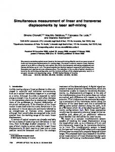
These formulae are valid for any angle of rotation φ, however, for the orthogonal regression, it is required to select such an angle that the joint moment. Thus, 2µ12 µ11 − µ22 2µ12 sin 2φ = p (µ11 − µ22 )2 + 4µ212 µ11 − µ22 cos 2φ = p (10) (µ11 − µ22 )2 + 4µ212 q 1 1 hX 2 i = (µ11 + µ22 ) + (µ11 − µ22 )2 + 4µ212 2 2 hXY i = 0 q Figure 1: The main screen of Polarobs. Measurements 1 1 hY 2 i = (µ11 + µ22 ) − (µ11 − µ22 )2 + 4µ212 of AM Her at the top and the background at the bot2 2 tom. In fact, there are four different roots φ = 12 arctan λ + kπ 2 , k = 0, 1, 2, 3 of the equation tan 2φ = λ. clicking and key pressing which is more comfortable Two of these four roots correspond to the direction when processing a large set of data. of the major axis of the dispersion ellipse along the OX When the data set is open, the program exhibits two axis while another two roots correspond to the direccurves which represent the resulted measurements of tion along the OY axis. We select the main direction in the object’s brightness (on the top of the screen) and the quadrant where the formulae for sin 2φ and cos 2φ sky background (on the bottom of the screen) for either are valid. Then, the variables X and Y have the highest of eight channels. Having the polynomial fitting of the and lowest dispersion, respectively, among all possible background counts performed the obtained polynomial angles of rotation. It is rather common that the varivalues are subtracted from the stars’ counts for each able X is interpreted as a variable parameter with the channel individually. Subsequently, the user can comobservation noise while Y is interpreted as ’pure noise’. pute the smoothing polynomial value for the reference The total Stokes parameters are calculated in the star counts in order to determine the brightness of the manner described. It follows from the above-presented target object. After that the program computes linformulae that using this technique the circular poear combinations (see 4) using fixed constants for each larization parameters are determined more precisely channel which results in the so-called ’vectors’ S1 − S4 . than those for the linear polarization. The first two vectors S1 and S2 are used later to compute the circular polarization parameters while another 3. Computer program two vectors (S3 and S4 ) are used to obtain the linear polarization parameters. Having this step completed, To process the observation data obtained with it is possible to save the results obtained in a format the single-channel photopolarimeter, Breus (2007) has of vectors of photometric observation, somehow similar written the computer program ”PolarObs”, which car- to the Stokes parameters. As the next step the user can analyse the diagram ries out the techniques described above (see also Breus representing the correlation between S2 and S1 (for the et al., 2007). A data file is generated by the telescope observa- circular polarization) and between S4 and S3 (for the tions; this file contains eight quasi-simultaneous mea- linear polarization). In this view mode the calculated surements of the object’s brightness for eight succes- values of polarization, position angle and other data sive positions of the modulator and the instant of time are shown under the diagram. When processing the standards of zero or non-zero at the end of a given observation. Information on the type of the object (such details as dark current, polarization, these data are considered to be and saved background, target star, reference star and standard), as the final results. When processing observations of exposure time and number of observation in a series a variable star or any other object it is necessary to and spectral band-filter is also recorded in the data file account for the instrumental polarization. To this end, by the polarimeter control program, written by a staff the coordinate system of the linear polarization diagram should be rotated by an angle determined from member of CrAO, D.N.Shakhovskoy. The program automatically identifies the type of the standards of non-zero linear polarization. data sequence using keyword analysis, giving the user To determine the circular polarization, it is necesthe option of accepting or changing the resulted type. sary to rotate the coordinate system of the circular Such a fashion allows of minimizing the amount of polarization diagram by a certain angle in such a way tan 2φ =

4

Odessa Astronomical Publications, vol. 29 (2016)

Figure 3: Viewing P-file - photometry (1), circular (2) and linear (3-4) polarization Figure 2: Diagram representing the correlation between S2 and S1 (left) and S4 and S3 (right) that the line connecting the origin and the distribution centre coincides with the OX axis. The standardised values of the Stokes parameters can be the output to the files with extension *.p on demand. These are delimited text files with spacebar and newline separated values which contain the following data: JD is the Julian date; Ft is the object brightness expressed as a ratio between the object counts and interpolated reference star count; Fm is the object brightness expressed in magnitude units (related to the Pogson formula Ft); CP1∗ , CP2∗ are the circular polarization values; LP1∗ , LP2∗ are the linear polarization values; σF , σCP , σLP are the errors in photometry, circular and linear polarization, respectively. In the last step it is possible to perform either polynomial approximation or averaging of the standardised or not-standardised Stokes parameters. When averaging, the program gives an option to select statistically optimal number of points for averaging using three test-functions, such as the estimated error of a single measurement, average accuracy of the smoothed value and the signal-to-noise ratio. The program was used to process the photopolarimetric observations of the stellar systems V405 Aur (Breus et al., 2013), BY Cam (Andronov et al., 2008), AM Her (Andronov et al., 2003) and QQ Vul (Andronov et al., 2010), as well as several comets (Kiselev et al., 2012; Rozenbush et al., 2007, 2009, 2014). Some results were reported in reviews on large scientific campaigns (Andronov et al., 2010; Vavilova et al., 2011, 2012).

References Andronov I.L. et al.: 2003, Odessa Astron. Publ., 16, 7. 2003OAP....16....7A Andronov I.L. et al.: 2008, Central European Journal of Physics, 6(3), 385. 2008CEJPh...6..385A Andronov I.L. et al.: 2010, Odessa Astron. Publ., 23, 8. 2010OAP....23....8A Breus V.V. : 2007, Odessa Astron. Publ., 20, 32. 2007OAP....20...32B Breus V.V., Andronov I.L., Kolesnikov S.V., Shakhovskoy N.M.: 2007, AATr, 26, 241. 2007A&AT...26..241B Breus V. V. et al.: 2013, JPhSt, 17, 3901. 2013JPhSt..17.3901B Kiselev N.N. et al.: 2012, LPI Contr. 1667, 6102. 2012LPICo1667.6102K Kucherov V.A.: 1986, KPCB, 2, 59. 1986KFNT....2...59K Rozenbush V.K. et al.: 2007, The 10-th Conference on Electromagnetic and Light Scattering, Bodrum, Turkey, Ed. by G.Videen et al. 2007Icar..186..317R Rozenbush V.K. et al.: 2009, Journal of Quantitative Spectroscopy and Radiative Transfer, 110 (14), p. 1719. 2009JQSRT.110.1719R Rosenbush V. et al.: 2014, Asteroids, Comets, Meteors, Helsinki, Finland. Edited by K. Muinonen et al., p. 450. 2014acm..conf..450R Serkowski K.: 1974. Planets, Stars and Nebulae, Studied with Photopolarimetry, ed. by Gehrels, Univ. of Arizona Press, Tucson, p. 135. 1974psns.coll..135S Shakhovskoy N.M. et al.: 2001, IzKry, 97, 91. 2001IzKry..97...91S Vavilova I.B. et al.: 2011, KosNT, 17, 74. 2011KosNT..17d..74V Vavilova I.B. et al.: 2012, KPCB, 28, 85. 2012KPCB...28...85V