Dhaka Univ. J. Sci. 60(2): 209-215, 2012 (July)
A Technique for Solving Special Type Quadratic Programming Problems M. Babul Hasan Department of Mathematics, University of Dhaka, Dhaka-1000, Bangladesh Email:
[email protected] Received on 20. 07. 2011. Accepted for Publication on 22. 02. 2012.
Abstract Because of its usefulness in production planning, financial and corporate planning, health care and hospital planning, quadratic programming (QP) problems have attracted considerable research and interest in recent years. In this paper, we first extend the simplex method for solving QP problems by replacing one basic variable at an iteration of simplex method. We then develop an algorithm and a computer technique for solving quadratic programming problem involving the product of two indefinite factorized linear functions. For developing the technique, we use programming language MATHEMATICA. We also illustrate numerical examples to demonstrate our technique.
Key Words: Quadratic programming, simplex method, algorithm, computer technique I. Introduction Non-linear Programming is a mathematical technique for determining the optimal solutions to many business problems. In a non-linear programming problem, either the objective function is non-linear, or one or more constraints have non-linear relationship or both. General Non-linear Programming Problem Let be a real valued function of variables defined (a)
Quadratic programming problem Let and matrix.Then,
.Let
be a symmetric
real
Maximize
,
Let
That is, quadratic programming is concerned with the NLPP of maximizing (or minimizing) the quadratic objective function, subject to a set of linear inequality constraints.
be a set of constraints such that
subject to the constraints
and
where and in a real matrix, is called a general quadratic programming problem.
(b)
Note: . .
represents a quadratic form.The reader may
recall that a quadratic form
is said to be positive-
definite (negative definite) if
for
and positive-semi-definite (negative-semi-definite) if satisfying where
are real valued functions of
variables
. Finally, let (c) xj ≥ 0.
j = 1, 2, ...
If either
.
is positive-semi-definite (negative-semi-
definite) then it is convex (concave) in and
over all of
,
or 2. If
some ; or both are non-linear, then the problem of determining the ntype which makes a maximum or minimum and satisfies (b) and (c), is called a general nonlinear programming (GNLP) problem. An NLP may be nonlinearly constrained or linearly constrained. If the objective of a linearly constrained NLP is a quadratic function then this problem is called quadratic programming (QP) problem. *Author for correspondence
such that there is one
It can easily be shown that 1. If
... ... .. m
for all
is positive-definite (negative-definite) then it is
strictly convex (strictly concave) in
over all of
.
These results help in determining whether the quadratic objective function is concave (convex) and the implication of the same on the sufficiency of the KarushKhun-Tucker conditioin for constrained maxima (minima) of .
210
M. Babul Hasan
Special type Quadratic programming problem
Where
In this chapter, we consider the quasi-concave quadratic programming problem (QP) subject to linear constraints as follows:
Let
are defined as in Section be the initial basic feasible solution to the (QP).
Then
where
,
(QP):Maximize subject to
Also let
,
where A =
, and
is a In addition we assume that
matrix, b
, x, c
,
. Here we
assume that
and Now let
and are positive for all feasible solution. (ii) The constraints set is non empty and bounded.
be another basic feasible solution where is the basis in which
(i)
In general, a quadratic programming problem is solved starting with some which satisfies the constraints but does not necessarily maximize
Then
replaced by are given by for
and
, and (Say) Where New optimizing value
where
In Section II, we present the simplex type method of Swarup [5] with numerical example. In Section III, we present our technique along with algorithm. We then conclude the paper in Section IV. Swarup’s Simplex Type Method for Solving QP Adding slack variables
to the
of (QP), we have the standard (QP) as Similary,
Maximize subject to
,
Hence ,
.Then the columns of
Then the new value of the basic variables in terms of the original ones and are as follows:
The rest of the paper is organized as follows.
(QPI):
but not in
is replaced by a series
of other (not necessarily basic feasible solutions) all of which satisfy the constraints until the required solution is obtained.There are many methods for solving (QP). Among them Wolf’s [4] method, Swarup’s [5] simplex type method and Gupta and Sharm’s [1] 2-basic variable replacement method are noteworthy. In this paper, we develop a computer technique for solving special type (quasi-concave) of QP problem in which the objective function can be factorized. Then compare the values of the objective function at these points in order to choose the optimal solution. We will introduce a computational technique to solve the QP problems by using computer algebra Mathematica [11].
constraints follows:
of
is
and
A Technique for Solving Special Type Quadratic Programming Problems
211
at a simplex table, the solution becomes optimal and the process terminates. Criterion1: (Choice of the entering variable) To identify the entering variable, choose the uth column of A for which is the greatest positive ; j = 1, 2,…, n
Optimality condition The value of the objective function will improve If
Criterion 2: (Choice of the outgoing variable) Choose
for which
Numerical Example Maximize But for non degenerate case subject to
,
,
, where Hence we must have,
Solution
Thus the solution can be improved until Whenever all
Introduction the slack variables to the constraints we get the initial table as follows:
for all for all
Table. 1. (Initial table) 2 1
0 0 0
0 0 0
4 1
1 2 0
3 1 1
1 2
0 0
0 0
0 0
0 0 4
1 0 0
0 1 0
0 0 1
2 1
4 1
1 3
0 0
0 0
0 0
3/2 8
4/3 43/3
¾ 11/2
-
-
-
b
4 3 3
212
M. Babul Hasan
Table.2
4 0 0
1 0 0
2 1
4 1
1 2
0 0
0 0
0 0
1/3 5/3 -1/3
1 0 0
0 0
1/3 -1/3 -1/3
0 1 0
0 0 1
b
4/3 5/3 5/3
4
2/3 2/3
0 0
1 62/9
1 2 -
-4/3 -1/3 5/12 101/6
0 0
0 0
4 -43/9
-
-
Table.3
4 0 0
1 0 0
2 1
4 1
1 2
0 0
0 0
0 0
1/3
1 0 0
0 0 1
1/3 -1/3 -1/12
0 1 0
0 0 1/4
-1/12 5/3
b
3/4 5/6
0 0
0 2
-5/4 -1/6
0 0
-1/4 -1/2
1 75/8
-
-
4 11/2
-
101/24 -
4/3 5/3 5/1
Table.4
4 2 1
1 1 2
2 1
4 1
1 2
0 0
0 0
0 0
0 1 0
1 0 0
0 0 1
2/5 -1/5 -1/10
-1/5 3/5 1/20
0 0 1/4
0 0
0 0
0 0
-11/10 0
-9/20 -1/2
-1/4 -1/2
-
-
-
5/2 -11/2
5/3 -45/8
2 -19/4
b
1 1 1/2
A Technique for Solving Special Type Quadratic Programming Problems
Since all
is non positive in Table-4, it gives the global
optimal solution. Hence the optimal solution is with global maximum,
Step 3: Test whether the linear system of equations has unique solution or not. Step 4: If the system of linear equations has got any unique solution, find it. Step 5: Dropping the solutions with negative elements, determine all basic feasible solutions.
.
III. Algorithm for Solving Special Type QP In this section, we present the computational technique for solving the QP problems. In 2000, Hasan et. al. [10] developed a computer oriented solution method for solving the LP problems. In this study, we will extend that method for solving the QP problems. We will see that, this method will help us to solve QP problems easily and to avoid the clumsy and time consuming methods of Swarup [5] and other methods. Step 1: Express the QP to its standard form. Step 2: Find all
sub-matrices of the coefficient
matrix
variables equal to zero.
by setting
213
Step 6: Calculate the values of the objective function for the basic feasible solution found in step 5. Step7: For the maximization of QP the maximum value of is the optimal value of the objective function, and the basic feasible solution which yields the optimal value is the optimal Solution. Computer code for solving special type QP In this section, we present our method for solving QP problems using computer algebra Mathematica.
214
INPUT:
OUTPUT:
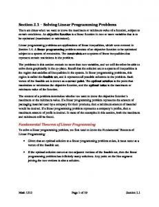
Graphical representation gives the actual concept of the problems. As, this is an optimization problem, we present graphical representation of this problem in the next section in order to achieve a more visual concept of the solutions of the given problem.
Graphical representation of numerical example of Section 2:
M. Babul Hasan
215
A Technique for Solving Special Type Quadratic Programming Problems
coefficient matrix A, right hand side constant b, cost coefficient vectors c and d and the constants and in the same program and easily obtained the optimal solution. Our method is also able to solve degenerate and cycling problems easily whereas the simplex method is proved to be inconvenient for solving such problems. IV. Conclusion In this paper, we developed a computer technique for solving special type (Quasi-Concave) of quadratic programming in which the objective function can be factorized. We illustrated the solution procedure developed by us with a numerical example. We observed that the result obtained by our procedure is completely identical with that of the other methods which are laborious and time consuming and clumsy. We therefore, hope that our program can be used as an effective tool for solving special type QP problems in which the objective function can be factorized and hence our time and labor can be saved. …………..
We observed that with Swarup’s [5] method we experienced complex calculations for the simplex tables. For solving problems with “ type” or “= type” constraints, one needs to solve that problem by Two-phase or Big-M simplex method which is clumsy and time consuming. But by our method, we just had to compute the
1.
Swarup, K., P. k. Gupta and Man Mohan, 2003,”Tracts in Operations Research”, Eleventh Thoroughly Revised Edition,ISBN:81-8054-059-6
2.
Frederick S. Hillier and Gerald J. Lieberman, McGraw-Hill International Edition 1995, ” Introduction to Operations Research”
3.
Wayne L. Winston, (1994), “Application and algorithms,” Dexbury press, Belmont, California, U.S.A.
4.
Wolfe, P., (1959), “The simplex method for quadratic programming,” Econometrica, 27(3), 382-398.
5.
Swarup, K. 1966, “Quadratic Programming” CCERO (Belgium), 8(2), 132-136.
6.
Swarup, K., 1964, “Linear fractional functional programming,” Operations Research, 13 (6), 1029-1036.
7.
Dantzig, G.B., 1962, “Linear programming and extension,” Princeton University press, Princeton,N.J.
8.
Hasan, M.B. and M.A.Islam, 2001, “Generalization of simplex method for solving fractional programming problems,” The Dhaka University Journal of Science, 53(1), 111-118.
9.
Hasan, M.B. (2008), “Solution of Linear Fractional Programming Problems through Computer Algebra”, The Dhaka University Journal of Science, 57(1),
10. Hasan, M. B., A.F.M.K Khan and M. A. Islam, 2001, “Basic solutions of linear system of equations through computer algebrs,” Ganit, Journal of Bangladesh Mathematical Society, 21 (1), 39-45. 11. Wolfram, S. 2000, “Mathematica,” Addision-Wesly Publishing Company, Melno Park, California, New York.