Remote Sens. 2015, 7, 8906-8924; doi:10.3390/rs70708906 OPEN ACCESS
remote sensing ISSN 2072-4292 www.mdpi.com/journal/remotesensing Article
A Temporal-Spatial Iteration Method to Reconstruct NDVI Time Series Datasets Lili Xu 1,2, Baolin Li 1,3,*, Yecheng Yuan 1, Xizhang Gao 1 and Tao Zhang 1,2 1
2 3
State Key Lab of Resources and Environmental Information System, Institute of Geographic Sciences and Natural Resources Research, CAS, Beijing 100101, China; E-Mails:
[email protected] (L.X.);
[email protected] (Y.Y.);
[email protected] (X.G.);
[email protected] (T.Z.) University of Chinese Academy of Sciences, CAS, Beijing 100049, China Jiangsu Center for Collaborative Innovation in Geographical Information Resource development and Application, Nanjing 210023, China
* Author to whom correspondence should be addressed: E-Mail:
[email protected]; Tel.: +86-010-6488-9072. Academic Editors: Raul Zurita-Milla and Prasad S. Thenkabail Received: 29 April 2015 / Accepted: 7 July 2015 / Published: 15 July 2015
Abstract: Reconstructing normalized difference vegetation index (NDVI) time series datasets is essential for monitoring long-term changes in terrestrial vegetation. Here, a temporal–spatial iteration (TSI) method was developed to estimate the NDVIs of contaminated pixels, based on reliable data. The NDVIs of contaminated pixels were first computed through linear interpolation of adjacent high-quality pixels in the time series. Then, the NDVIs of remaining contaminated pixels were determined based on the NDVI of a high-quality pixel located in the same ecological zone, showing the most similar NDVI change trajectories. These two steps were repeated iteratively, using the estimated NDVIs as high-quality pixels to predict undetermined NDVIs of contaminated pixels until the NDVIs of all contaminated pixels were estimated. A case study was conducted in Inner Mongolia, China. The accuracies of estimated NDVIs using TSI were higher than the asymmetric Gaussian, Savitzky–Golay, and window-regression methods. Root mean square error (RMSE) and mean absolute percent error (MAPE) decreased by 16.7%–86.6% and 18.3%–33.0%, respectively. The TSI method performed better over a range of environmental conditions, the variation of performance by the compared methods was 1.4–5 times that of the TSI method. The TSI method will be most applicable when large numbers of contaminated pixels exist.
Remote Sens. 2015, 7
8907
Keywords: reconstruction; time series; NDVI; trajectory distance; temporal-spatial correlation
1. Introduction The normalized difference vegetation index (NDVI) is an important indicator of vegetation status [1,2]. NDVI time series datasets have been used to identify phenological characteristics, for monitoring long-term trends, for detecting abrupt changes and in multi-temporal classification [3–6]. However, pixels contaminated by atmospheric conditions, sensor viewing angles, or variations in sun-surface-sensor geometry always exist in an NDVI time series dataset [7–9]. It is important to determine the “accurate” NDVI values of contaminated pixels because inaccurate NDVIs can result in a misinterpretation of the dynamics of terrestrial ecosystems [10,11]. Wessels et al. (2007) stated that a 15% NDVI reduction at different locations in the time series indicated a clear difference in the NDVI trend [12]. Therefore, the reconstruction of accurate time series datasets is essential for the use of Moderate Resolution Imaging Spectroradiometer (MODIS) MODIS13Q1, National Oceanic and Atmospheric Administration (NOAA) Global Inventory Modeling and Mapping Studies (GIMMS), NOAA Pathfinder (PAL), or Systeme Probatoire d’Observation de la Terre (SPOT) Vegetation (VGT) NDVI datasets. Much research in recent years has been conducted on methods for reconstructing NDVI datasets that contain contaminated pixels. Most methods, such as the Savitzky–Golay (SG) [13,14], mean value iteration [15], best index slope extraction [16], double logistic [17], asymmetric Gaussians (AG) [18], and Fourier analysis [19] methods, have been applied to determine the values of contaminated pixels based on the integrality and consistency of the entire time series dataset, according to either the frequency or the temporal domain [20,21]. However, continuously contaminated pixels appear quite frequently in the NDVI series, and the use of a limited number of high-quality pixels to establish these values can result in poor model performance. To overcome this problem, alternative methods have been developed to determine the values of contaminated pixels based on the correlation of data within the spatial dimension combined with the temporal dimension [22]. Cho and Suh [23] used a land cover map for 2006–2008 to define the spatial neighborhood, and estimated the NDVIs of contaminated pixels by weighting the NDVIs of high-quality pixels that had the same land cover type within a predetermined window. However, it is difficult to obtain highly accurate land cover maps: for example, the global land cover map based on Thematic Mapper/Enhanced Thematic Mapper Plus (TM/ETM+) data has accuracy of only about 65% [24,25]. Low-accuracy land cover maps can result in high uncertainty in the estimated NDVIs of contaminated pixels. De Oliveira et al. [20] proposed a spatial-temporal window method, window-regression (WR), to estimate the NDVI of a contaminated pixel through regression analysis between the NDVIs of the contaminated pixel and others within a predetermined window. However, contaminated pixels are frequently aggregated and, if there is a lack of high-quality pixels within the predetermined window, contaminated NDVIs cannot be estimated. Furthermore, if there are many regression equations with low reliability, there will be high uncertainty regarding the integrity of the estimated NDVIs.
Remote Sens. 2015, 7
8908
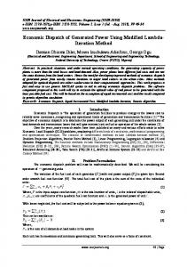
As discussed above, two fundamental problems need to be addressed when using a method based on spatial estimation. The first is to define a temporal–spatial neighborhood that can estimate all the contaminated NDVIs. Second, a means by which to estimate the NDVIs of the contaminated pixels without reference to existing land cover maps should be established. Here, to overcome these two problems, a temporal-spatial iteration (TSI) method is proposed that estimates the NDVIs of the contaminated pixels based on temporal-spatial neighborhood estimation without reference to land cover maps or to an arbitrary predetermined window. In this study, we took an ecological zone as the spatial neighborhood to obtain high-quality NDVIs from the same land cover types. We estimated the NDVIs of the contaminated pixels using the NDVIs of high-quality pixels that reflected similar land cover types. This was achieved using the weighted trajectory distance (WTD) algorithm based on NDVI change trajectories, which avoided the need to use existing land cover maps. 2. Materials and Methods 2.1. Study Area The study areas were within the Inner Mongolian Autonomous Region of China (37°24′–53°23′N, 97°12′–126°04′E), which covers about 1,180,000 km2 and consists of 89 banners (counties or cities). The natural environment of the study area is strongly heterogeneous. Annual precipitation varies from 50 mm/a in the northwest to 500 mm/a in the northeast. Annual average temperature varies from 0 to 8 °C. Humid, semiarid, and arid zones are found from east to west, respectively. Soil types are black soil, chernozem, chestnut soil, and sandy soil. Vegetation comprises forest, steppe, desert-steppe, and desert. Nine sub-areas were chosen (Figure 1), three from each of the humid, semiarid, and arid zones. MODIS images of each sub-area covered 2500 km2 and comprised 40,000 pixels (i.e., 200 rows × 200 columns). Sub-areas 1–3 were in a typical humid region, located in northeast of the main study area where the dominant land cover was forest. Sub-areas 4–6 were in a typical semiarid region with mainly grassland cover, located in the middle of the study area. Sub-areas 7–9 were located in the west of the study area, a typical arid region with vegetation cover of sparse forest or shrubland. The geographic coordinates of the center pixels of the nine sub-areas are listed in Table 1. Table 1. Location of the nine selected sub-areas. Study Area Humid area
Semi-arid area
Arid area
Sub-area 1 Sub-area 2 Sub-area 3 Sub-area 4 Sub-area 5 Sub-area 6 Sub-area 7 Sub-area 8 Sub-area 9
Geographic Coordinates of the Center Pixel 50°22′112′′N, 121°1′40′′E 49°26′33′′N, 123°38′54′′E 48°27′57′′N, 120°55′56′′E 44°51′11′′N, 118°40′11′′E 43°18′31′′N, 118°50′25′′E 42°24′22′′N, 115°7′4′′E 40°45′8′′N, 106°28′8′′E 40°11′55′′N, 104°2′52′′E 40°54′33′′N, 103°57′8′′E
Remote Sens. 2015, 7
8909
Figure 1. Location of the study area and nine selected sub-areas. 2.2. Data and Data Preprocessing The NDVI time series data were taken from MODIS13Q1 datasets downloaded from the MODIS website (http://modis.gsfc.nasa.gov/), covering 92 dates from 2010 to 2013. Data from layer 1 and layer 12 of the MODIS13Q1 dataset were used in this study. Layer 1 reflects the NDVI value and layer 12 provides information on the reliability and quality of the pixel data for each pixel in the dataset. Both layers have the same temporal resolution (16 days) and spatial resolution (250 m). They were reprojected to Albers equal area projection with a WGS84 datum using the MODIS Reprojection Tool (MRT) and the nearest neighbor resampling method. The 1:5,000,000 ecological map of Inner Mongolia was used to identify ecological zones. An ecological zone is determined by the climate, soil, landform and vegetation. In an ecological zone, the combination of land cover types is unique and is similar in its different sub-areas. The same kind of land cover type in an ecological zone indicates the similar combination of plants and their growing processes. The values of pixel reliability of the MODIS13Q1 dataset were classified into five ranks [3]: “−1” indicated the corresponding pixel was not processed and that it should be treated as null; “0” indicated the corresponding pixel was good with high-quality data; “1” indicated the value of the corresponding pixel was marginal but that it could be used with reference to other quality assurance information; “2” indicated the targets in the corresponding pixel were covered with snow or ice when the data were produced; and “3” indicated the targets in the corresponding pixel were invisible (usually because of cloud cover). The NDVIs of pixels with rankings of “−1”, “2”, and “3” were considered unreliable and defined as “contaminated” pixels. The NDVI datasets were then classified into high-quality pixels (group 1) and contaminated pixels (group 2).
Remote Sens. 2015, 7
8910
According to a statistical analysis of the NDVI dataset in the study area, 65.4% and 14.0% of pixels were classified as groups “0” and “1”, respectively, and 11.8% and 8.7% of pixels were classified as groups “2” and “3”, respectively. Only