A tensorial approach to computational continuum mechanics using object-oriented techniques H. G. Weller and G. Tabora! Department of Mechanical Engineering, Imperial College, London SW7 2BX, United Kingdom H. Jasak Computational Dynamics Limited, London W10 6RA, United Kingdom C. Fureby Department of Weapons and Protection, National Defense Research Establishment (FOA), S-17290 Stockholm, Sweden (Received 1 June 1998; accepted 13 August 1998)
In this article the principles of the field operation and manipulation ~FOAM! C11 class library for continuum mechanics are outlined. Our intention is to make it as easy as possible to develop reliable and efficient computational continuum-mechanics codes: this is achieved by making the top-level syntax of the code as close as possible to conventional mathematical notation for tensors and partial differential equations. Object-orientation techniques enable the creation of data types that closely mimic those of continuum mechanics, and the operator overloading possible in C11 allows normal mathematical symbols to be used for the basic operations. As an example, the implementation of various types of turbulence modeling in a FOAM computational-fluid-dynamics code is discussed, and calculations performed on a standard test case, that of flow around a square prism, are presented. To demonstrate the flexibility of the FOAM library, codes for solving structures and magnetohydrodynamics are also presented with appropriate test case results given. © 1998 American Institute of Physics. @S0894-1866~98!01906-3#
INTRODUCTION
where
Computational continuum mechanics ~CCM! is the simulation of continua using computers. Fluid dynamics is a significant branch of continuum mechanics and covers a variety of cases, including compressible, incompressible, multiphase, and free-surface flows, as well as flows involving further physics such as chemical reactions, species transport, phase changes, and electromagnetic effects. All these flows can be described by systems of linked partial differential equations of the form
]r Q 1¹–~ r U ^ Q! 2¹–r D¹Q5S p Q1S q , ]t
~1!
where U is the fluid velocity, r its density, and Q is any tensor-valued property of the flow, such as species concentration. These equations involve time derivatives ( ]r Q/ ] t), convective terms @ ¹–( r U ^ Q) # , diffusive terms (¹–r D¹Q), and source terms ~SQ and S q !. A simple example is that of incompressible flow as described by the Navier–Stokes equations (Q5 $ 1,U% ): ¹–U50,
]U 1 1¹–~ U ^ U! 2¹–2 n D52 ¹ p, ]t r a!
Corresponding author; E-mail:
[email protected]
620
COMPUTERS IN PHYSICS, VOL. 12, NO. 6, NOV/DEC 1998
~2!
D5 21 ~ ¹U1¹UT ! .
~3!
The effect of the nonlinearity embodied in these equations is significant; only in special cases can algebraic solutions be found. The vast majority of fluid-flow problems can only be properly studied by using computational methods involving discretization of the domain and the equations, followed by numerical solution of the resulting system of equations. The complexity of the problem is increased if effects such as turbulence, compressibility, multiphase, free surface, chemical reactions, and electromagnetism are included. The two predominant solution techniques are the finite-element method ~FEM!,1 in which the functional form of the solution to these equations is expanded in terms of a predetermined basis set and its residual minimized, and the finite-volume method ~FVM!.2,3 In the latter technique, which is used in this article, the computational domain is divided into a set of discrete volumes d V i which fill the computational domain D without overlap, i.e., ø i d V i 5D and ù i d V i 5B. The fluid-flow equations are then volumeintegrated over each individual finite volume d V i . Gauss’s theorem is used to convert the divergence terms in Eqs. ~2! into surface-integrated flux terms, reducing the problem of discretizing these terms to one of finding difference approximations for the fluxes at the surface of the control volume based on the known cell-center values. Other spatial derivatives are dealt with in a similar manner. This © 1998 AMERICAN INSTITUTE OF PHYSICS 0894-1866/98/12~6!/620/12/$15.00
converts the equations into a set of ordinary differential equations including temporal derivatives, which can be discretized in a straightforward manner using finite-difference approximations. This results in a set of difference equations that, when linearized by fixing the flux rU, can be described in matrix form Mc 5y,
~4!
where M is a sparse block matrix: this can be inverted to solve the equation. The nonlinear term in Eqs. ~2! requires an iterative solution technique, one in which the linearized system specified above is solved several times, with the fluxes being updated each time, until it has converged sufficiently. Coupling between equations is treated in field operation and manipulation ~FOAM! using a segregated approach, in which equations are formulated for each dependent variable and solved sequentially, with the possibility of iteration over the system of equations until convergence is achieved. So, for example, any vector equation is solved by solving each component in turn as a scalar equation, within the solution of the overall vector equation ~i.e., the user sees a vector equation, but when the solution actually occurs, the components are solved for sequentially!. Provided that the coupling between the components is not strong ~as it would be if the coupling were due to a cross product of some form!, this is quite acceptable. If the need arises, the design of FOAM does not preclude the implementation of a block solver to solve the components of a vector ~or tensor! equation simultaneously. In general, CCM and computational-fluid-dynamics ~CFD! codes have been written in procedural languages, in particular in Fortran.2 This reliance on procedural programming techniques has led to a concentration on the lower levels of the coding: implementation of models, however complicated, is often discussed in terms of the manipulation of individual floating-point values. The approach presented in this article is different and has culminated in the creation of the FOAM C11 class library for CCM. The intention is to develop a C11 class library that makes it possible to implement complicated mathematical and physical models as high-level mathematical expressions. This is facilitated by making the high levels of the code resemble as closely as possible standard vector and tensor notation. In this approach the tensorial fields Q5 r , U, etc., which represent the state of the system of interest, are considered as the solution of a set of partial differential equations ~PDEs! ~2!, rather than viewing the problem as a numerical one in which arrays of floating values are obtained by inverting matrices. An object-oriented programming ~OOP! methodology has been adopted for this approach. It is generally recognized that OOP produces code that is easier to write, validate, and maintain than procedural techniques.4 Our intention in this article is to demonstrate the utility of OOP techniques for solving continuummechanics ~and especially fluid-dynamics! problems. The exact definition of an OOP language is a matter that is discussed elsewhere,5,6 but Stroustrup suggests that an OOP approach is one that involves abstraction, inheritance, and polymorphism.7 Abstraction is the ability to represent conceptual constructs in the program and to hide details behind an interface. This is achieved by allowing the programmer to create classes to represent conceptual ob-
jects in the code, classes that encapsulate, i.e., contain and protect, the data that make up the object. Member functions are provided that permit limited, well-defined access to the encapsulated data. Thus it is possible to create data types that represent tensor fields ~see Sec. I A! and typical terms in the equations constructed to behave like their mathematical counterparts ~Sec. I B!, hiding the numerical details of the implementation by encapsulation. The class interface is designed to resemble standard mathematical notation, as seen below, while the implementation is not relevant at this level. Inheritance enables relationships between the various classes to be expressed, representing commonality between different classes of objects by class extension. By doing this existing classes can be given new behavior without the necessity of modifying the existing class. For example, this can be used to construct a complicated mathematical class by extending base classes that express simpler mathematical objects. A class representing the algebraic structure of a ring could thus be derived from a pre-existing group class by adding the concept of multiplication. Examples of this within FOAM include the use of inheritance to represent conceptual links between turbulence models ~see Sec. II!. Polymorphism is the ability to provide the same interface to objects with different implementations, thus representing a conceptual equivalence between classes that in practical terms have to be coded differently. Examples of this in FOAM include the implementation of boundary conditions ~Sec. I C!. C11 is a good programming language for scientific work; although it is less rigorously object-oriented than other languages such as Smalltalk or Eiffel, there are practical considerations to take into account. Its author, Stroustrup, intended it to support a range of programming styles, and so he incorporated a number of conceptual tools, not all of which are strictly object-based. In particular, C11 implements operator overloading, which is essential in order to construct an interface that resembles standard mathematical notation. Moreover it is widely available on all platforms and, being based on C, is fast. Recent studies8,9 indicate no significant difference in performance between Fortran and the C group of languages. In this article C11 terminology is adopted when discussing OOP, and so reference is made to member functions and multiple inheritance, rather than to methods and interfaces. While a great deal of attention has been paid to the development of new and efficient algorithms for CFD, little has been published about overall code design. Some work has been done on the use of object-oriented methods in the FEM10,11 and in the spectral-element method.12 The approach has tended to be from the perspective of linear algebra in which the highest-level data structures represent vectors and matrices, although there have been some attempts to develop symbolic-manipulation techniques within OOP to derive and automatically code matrix forms for structural calculations.13,14 The approach proposed here, which is from the viewpoint of the tensor calculus, is considered appropriate for the FVM and is easier to understand from the point of view of the continuum mechanics. The result is a C11 class library in which it is possible to implement a wide variety of continuum-mechanics modeling techniques, including those of incompressible and compressible fluid flow,15 multiphase flow, and free surface flow,16 together with various turbulence modeling COMPUTERS IN PHYSICS, VOL. 12, NO. 6, NOV/DEC 1998
621
techniques.17 In fact any system of time-dependent PDEs including convection, diffusion, and source terms can be handled. In this article an outline of the library is presented and discussed, including some of the issues involved in our approach to implementing classes for tensor fields and differential equations. These issues are illustrated by reference to the two main modeling techniques for turbulent flow: Reynolds-averaged simulation and large-eddy simulation, which are implemented as virtual class hierarchies. Results are presented for the simulations of incompressible flow around a square prism. To illustrate the flexibility of the code, two other examples are also presented, one involving magnetohydrodynamical flow in a duct, and the other the calculation of the stress and strain fields in an elastic solid. I. IMPLEMENTATION A. Implementation of tensor fields The majority of fluid dynamics can be described using the tensor calculus of up to rank 2, i.e., scalars, vectors, and second-rank tensors. Therefore three basic classes have been created: scalarField, vectorField, and tensorField. Details of the implementation of these field classes will be described in a future paper; in this article we concentrate on the code-design issues relating to the tensor-field interface and the differential operators thereof. One of the great advantages of OOP is that this division into interface versus implementation is possible: in theory, it should be possible to rewrite totally the tensor implementation without affecting the rest of the library.18 These tensor field classes are somewhat different from a mathematical tensor field in that they contain no positional information; they are essentially ordered lists of tensors, and so only pointwise operations ~i.e., tensor algebra! can be performed at this level. The operators implemented include addition and subtraction, multiplication by scalars, formation of various inner products, and the vector and outer products of vectors ~resulting in vectors and tensors, respectively!. In addition, operations such as taking the trace and determinant of a tensor are included as well as functions to obtain the eigenvalues and eigenvectors; these are not necessary for solution of fluid systems but are of importance for postprocessing the data ~see comments below!. Since C11 implements operator overloading, it is possible to make the tensor algebra resemble mathematical notation by overloading 1, 2, !, etc. The one problem inherent here is that the precedence of the various operators is preset, which makes it quite difficult to find an operator for the dot product with the correct precedence and that looks correct. The next level of tensors are referred to as ‘‘geometric tensor fields’’ and contain the positional information lacking in the previous classes. Again, there are classes for the three ranks of tensors currently implemented, volScalarField, volVectorField, and volTensorField. At first, the relationship between, for example, scalarField and volScalarField should be ‘‘isA,’’ i.e., derivation. However, this would allow the compiler to accept scalarField1volScalarField as an operation, which would not be appropriate, and so encapsulation is used instead. In addition to the additional metrical information necessary to perform differentiation, which is contributed by a reference 622
COMPUTERS IN PHYSICS, VOL. 12, NO. 6, NOV/DEC 1998
to a ‘‘mesh class’’ fvMesh ~see below!, these classes contain boundary information, previous time steps necessary for the temporal discretization, and dimension set information. All seven base SI dimensions are stored, and all algebraic expressions implemented above this level are dimensionally checked at execution. It is therefore impossible to execute a dimensionally incorrect expression in FOAM. This has no significant runtime penalty whatsoever: typical fields have 104 – 105 tensors in them, and dimension checking is done once per field operation. Currently two types of tensor-derivative classes are implemented in FOAM: finiteVolumeCalculus or fvc, which performs an explicit evaluation from predetermined data and returns a geometric tensor field, and finiteVolumeMethod or fvm, which returns a matrix representation of the operation, which can be solved to advance the dependent variable~s! by a time step. fvm will be described in more detail in Sec. I B. The fvc class has no private data and merely implements static member functions that map from one tensor field to another. Use of a static class in this manner mimics the concept of a namespace which has recently been introduced into C11, and by implementing the operations in this manner, a clear distinction is drawn between the data and the operations on the data. The member functions of this class implement the finite-volume equivalent of various differential operators, for example, the expression vorticity 5 0.5*fvc::curl(U);
calculates the vorticity of a vector field U as 21 ¹3U. 1 ~For reasons of space, not all the variables in the program fragments used to illustrate points will be defined. The names are, however, usually quite descriptive.! This also illustrates the ease with which FOAM can be used to manipulate tensorial data as a postprocessing exercise. Any FOAM code can be thought of as an exercise in mapping from one tensor field to another, and it matters little whether the mapping procedure involves the solution of a differential equation or not. Hence, writing a short code to calculate the vorticity of a vector field is a matter of reading in the data ~for which other functions, not described here, are provided!, performing this manipulation, and writing out the results. Very complicated expressions can be built up in this way with considerable ease. All possible tensorial derivatives are implemented in FOAM: ] / ] t, ¹–, ¹, and ¹3. In addition, the Laplacian operator is implemented independently rather than relying on the use of ¹ followed by ¹–. This enables improved discretization practices to be used for this operator. The one numerical issue that has to be dealt with at the top level of the code is the choice of differencing scheme to be used to calculate the derivative. Again, because of the data hiding in OOP, the numerics can be effectively divorced from the high-level issues of modeling: improved differencing schemes can be implemented and tested separately from the codes that they will eventually be used in. The choice can be made at the modeling level by using a switch in the operator. Hence, the temporal derivative ] / ] t can be invoked as volVectorField dUdt 5 fvc::ddt(U, EI)
where the second entry specifies which differencing
scheme to use ~in this case Euler implicit!. Several temporal differencing schemes are available, with a default corresponding to the scheme that gets the most use, in this case, backward differencing. Other selection methods are possible, but this one is the simplest. B. Implementation of partial-differential-equation classes The fvc methods correspond directly to tensor differential operators, since they map tensor fields to tensor fields. CCM requires the solution of partial differential equations, which is accomplished by converting them into systems of difference equations by linearizing them and applying discretization procedures. The resulting matrices are inverted using a suitable matrix solver. The differential operators ¹–, ¹, and ¹3 lead to sparse matrices, which for unstructured meshes have a complex structure requiring indirect addressing and appropriate solvers. FOAM currently uses the conjugate-gradient method,19 with incomplete Cholensky preconditioning ~ICCG!,20 to solve symmetric matrices. For asymmetric matrices the Bi-CGSTAB method21 is used. The matrix inversion is implemented using face addressing throughout,15 a method in which elements of the matrix are indexed according to which cell face they are associated with. Both transient and steady-state solutions of the equation systems are obtained by time-marching, with the time step being selected to guarantee diagonal dominance of the matrices, as required by the solvers. In order that standard mathematical notation can be used to create matrix representations of a differential equation, classes of equation object called fvMatrixScalar, fvMatrixVector, etc., are defined to handle addressing issues, storage allocation, solver choice, and the solution. These classes store the matrices that represent the equations. The standard mathematical operators 1 and 2 are overloaded to add and subtract matrix objects. In addition, all the tensorial derivatives ] / ] t, ¹–, ¹3, etc., are implemented as member functions of a class finiteVolumeMethod ~abbreviated to fvm!, which construct appropriate matrices using the finite-volume discretization. Numerical considerations are relevant in deciding the exact form of many of the member functions. For instance, in the FVM, divergence terms are represented by surface integrals over the control volumes d V i . Thus the divergence function call is div(phi,Q), where phi is the flux, a field whose values are recorded on the cell faces, and Q is the quantity being transported by the flux, and is a field whose values are on the cell centers. For this reason, this operation cannot be represented as a function call of the form div(phi*Q). Again, the Laplacian operator is implemented as a single separate call rather than as calls to div and grad, since its numerical representation is different. Various forms of source term are also implemented. A source term can be explicit, in which case it is a special kind of equation object with entries only in the source vector y, or it can be made implicit, with entries in the matrix M. In Eq. ~1! these are the terms S q and S p Q, respectively. Construction of an explicit source term is provided for by further overloading 1 ~and 2! to provide operations such as fvm1volScalarField. Construction of an implicit source is arranged by providing a function Sp(a,Q), thus specifying the dependent variable Q to be solved for.
Thus it is possible to build up the matrix system appropriate to any equation by summing the individual terms in the equation. As an example, consider the mass conservation equation ]r / ] t1¹–( f )50, where f 5 r U. The matrix system can be assembled by writing fvMatrixScalar rhoEq ( fvm::ddt(rho) 1 fvc::div(phi) );
where the velocity flux phi has been evaluated previously, and solved by the call rhoEq.solve( );
to advance the value of r by one timestep. Where necessary, the solution tolerance can be explicitly specified. For completeness, the operation 55 is defined to represent mathematical equality between two sides of an equation. This operator is here entirely for stylistic reasons, since the code automatically rearranges the equation ~all implicit terms go into the matrix, and all explicit terms contribute to the source vector!. In order for this to be possible, the operator chosen must have the lowest priority, which is why 55 was used; this also emphasizes that this represents equality of the equation, not assignment. C. Mesh topology and boundary conditions Geometric information is contributed to the geometric fields by the class fvMesh, which consists of a list of vertices, a list of internal cells, and a list of boundary patches ~which in turn are lists of cell faces!. The vertices specify the mesh geometry, whereas the topology of any cell—be it one dimension ~1D! ~a line!, two dimensions ~2D! ~a face!, or three dimensions ~3D! ~a cell!—is specified as an ordered list of the indices together with a shape primitive describing the relationship between the ordering in the list and the vertices in the shape. These primitive shapes are defined at run time, and so the range of primitive shapes can be extended with ease, although the 3D set tetrahedron ~four vertices!, pyramid ~five vertices!, prism ~six vertices!, and hexahedron ~eight vertices! cover most eventualities. In addition, each n-dimensional primitive shape knows about its decomposition into (n21)-dimensional shapes, which are used in the creation of addressing lists as, for example, cell-to-cell connectivity. Boundary conditions are regarded as an integral part of the field rather than as an added extra. fvMesh incorporates a set of patches that define the exterior boundary ] D of the domain. Every patch carries a boundary condition, which is dealt with by every fvm operator in an appropriate manner. Different classes of patch treat calculated, fixed value, fixed gradient, zero gradient, symmetry, cyclic, and other boundary conditions, all of which are derived from a base class patchField. All boundary conditions have to provide the same types of information, that is, that they have the same interface but different implementations. This is therefore a good example of polymorphism within the code. From these basic elements, boundaries suitable for inlets, outlets, walls, etc., can be devised for each specific situation. An additional patchField, processor is also available. Parallelization of FOAM is via domain decomposiCOMPUTERS IN PHYSICS, VOL. 12, NO. 6, NOV/DEC 1998
623
tion: the domain is split into N subdomains, one for each processor available at run time, and a separate copy of the code is run on each domain. However, separate processors need to exchange information within the solver, and this is the function of the processor patch class. On decomposition, internal boundaries within the ~complete! mesh are given processor patches, which know about the interprocessor topology and hide the interprocessor calls. ~At the bottom level, PVM, MPI, or SHMEM calls can be used, depending on the computer, without affecting the rest of the code.! This has the additional benefit that, since the interprocessor communication is at the level of the field classes, any geometric field, and hence any FOAM code, will automatically parallelize. Other than this, the parallelization behaves in the expected manner, showing linear speedup for a small number of processors and becoming less efficient when the number of processors involved is increased ~that is, when message passing becomes a critical factor!.
D. An example: icoFoam As an example, the following is the main part of a code, icoFoam, which solves the incompressible Navier–Stokes Eqs. ~2!. The predictor–corrector PISO method,22,23 in which the pressure and velocity fields are decoupled and solved iteratively, is as follows. ~1! An initial guess for the pressure field is made ~in fact, the pressure solution from the previous time step is used! and the momentum equation is solved to a predefined tolerance to give an approximate velocity field. ~2! The pressure Poisson equation is then formulated with the divergence of the partial velocity flux as a source term and solved to give a new estimate of the pressure field. A new set of conservative fluxes is obtained from the pressure equation. ~3! The corrected pressure field is used in an explicit correction to the velocity field. Steps ~2! and ~3! can be iterated as many times as are necessary to reach a converged solution. Usually two PISO correctors are sufficient for each time step, although this is dependent on the time step selected, which in turn depends on the temporal accuracy required. for(runTime11; !runTime.end( ); runTime11) $ Info ! ‘‘Time 5 ’’ ! runTime.curTime( ) nl ! endl; fvMatrixVector Ueqn ( fvm::ddt(U) 1fvm::div(phi, U) 2fvm::laplacian(nu, U) ); solve(Ueqn 55 2 fvc::grad(p)); // --- PISO loop for (int corr 5 0; corr,nCorr; corr11) $ phi 5 Interpolate(Ueqn.H( )/Ueqn.A( )) & mesh.areas( ); fvMatrixScalar peqn ( fvm::laplacian (1.0/Ueqn.A( ), p) 55 fvc::div(phi) 624
COMPUTERS IN PHYSICS, VOL. 12, NO. 6, NOV/DEC 1998
); peqn.setReference(0, 0.0); peqn.solve( ); phi 2 5 peqn.flux( ); U 5 (Ueqn.H( ) 2 fvc::grad(p))/Ueqn.A( ); U.correctBoundaryConditions( ); %
%
II. TURBULENCE MODELING A major issue in fluid dynamics is the existence of turbulence. In a turbulent flow, there are coherent structures on a variety of spatial scales from the largest, determined by the size of the geometry, down to very small scales where viscous effects dominate. The range of scales involved may be over several decades. There are two approaches to solving for turbulence: either the mesh used is fine enough to resolve ~and thus simulate! all of the flow scales, or the range of scales explicitly simulated must be reduced, with the effect of the unresolved scales being accounted for by modeling. In Reynolds-averaged simulations ~RAS!, the flow is decomposed into an average part and a fluctuating part, where the averaging can be across an ensemble of equivalent flows, or can be a time average over a time d t, short in comparison to any long-term changes to the flow but long compared to the turbulent fluctuations. In all cases the de¯ composition of the velocity field may be written U5U 1U8 , where the overbar indicates the average and the prime the fluctuating component. Applying this averaging to the momentum equation ~2! yields ¯ ]U 1 ¯ ^U ¯ ! 1¹–R2¹–2 n D ¯ 52 ¹ ¯p 1¹–~ U ]t r
~5!
where R5U8 ^ U8 is the Reynolds stress tensor. R is commonly modeled as a turbulent viscosity n t times “U, and n t evaluated from a hierarchy of equations derived from nth order moments of the Navier–Stokes equation ~NSE!. These are also commonly referred to as algebraic stress models. As an alternative, dynamic equations for R can be formulated; these contain terms including triple correlations of the fluctuating velocity, which must be modeled. Such models, known as Reynolds Stress ~RS! models, involve much more effort in their solution, since, although R is a symmetric tensor, it still has six independent components to be solved for, and the equation set is even stiffer than that for the standard k2 e model. A completely different approach is that of large-eddy simulation ~LES!, in which the division is by scale via a filtering operation that can be conveniently represented as a convolution between the dependent field variable and a filter function with particular properties. The filtered form of the NS equations is ¯ 50, ¹–U ¯ 1 ]U ¯ ^U ¯ ! 1¹–B2¹–2 n D ¯ 52 ¹ ¯p , 1¹–~ U ]t r
~6!
where B is the subgrid scale ~SGS! stress tensor ¯ ^U ¯. B5U ^ U2U
~7!
Turbulence modeling consists of finding convenient and physically correct representations for R and B. A. RAS modeling In all there are 11 RAS models implemented in FOAM, including standard,24 nonlinear, and low-Reynoldsnumber25 variants of the k2 e model, q2 z , and nonlinear Shih models. The appropriate terms and equations can be incorporated directly into the code as additions to the NSE. However, since FOAM is intended as a research tool for investigating fluid flows as well as modeling, it is important to be able to select the turbulence model at run time without recompiling the code. Once again, OOP techniques are of value here. Since all of the models generate a term of the form “–R to add to the momentum equation, they can be implemented as a set of classes with a common interface. This implies that polymorphism via a virtual class hierarchy is appropriate. A virtual base class turbulenceModel is declared, and classes that implement the various RAS models are derived from it. The model selection is stored in a parsed dictionary file, and a pointer mechanism is used to instantiate the correct RAS model as an instance of the virtual base class turbulenceModel at run time, with the values of the coefficients being taken from this file as well. The additional terms can be included into the averaged NSE as follows: fvMatrixVector Ueqn ( fvm::ddt(U) 1 fvm::div(phi, U) 2 fvm::laplacian(turbulence.nuEff( ), U) 1 turbulence.momentumSource( ) ); solve (Ueqn 55 2 fvc::grad(p));
¯ u2, P k 52 n t u ¹U ~8!
]e n e e2 ¯ e ! 2¹– t ¹ e 5C 1 e P k 2C 2 e , 1¹–~ U ]t se k k where P k is the production rate of k and s k , s k , C 1 e , and C 2 e are model coefficients. Below is an example of how this can be implemented in FOAM. // Turbulent kinetic energy production volScalarField Pk 5 2*nut*magSqr(fvc::grad(U)); // Turbulent kinetic energy equation solve ( fvm::ddt(k) 1 fvm::div(phi, k) 2 fvm::laplacian(nu/sigmaK, k) 55
Pk 2 fvm::Sp(epsilon/k, k) ); // Dissipation equation solve ( fvm::ddt(epsilon) 1 fvm::div(phi, epsilon) 2 fvm::laplacian(nu/sigmalEps, epsilon) 55 C1*Pk*epsilon/k 2 fvm::Sp(C2*epsilon/k, Epsilon) );
Reynolds stress models can be implemented in a similar manner. Here, for example, is the implementation of the Launder–Reece–Rodi ~LRR! model equation26 for the Reynolds stress tensor R:
where turbulence is the RAS-model object. The contribution of the turbulence model to the flow is via the member function nuEff(), which returns n 1 n t , where n is the laminar viscosity. As an example, the standard k2 e model24 requires the solution of the following equations for turbulent kinetic energy k and dissipation rate e:
]k n ¯ k ! 2¹– t ¹k5 P k 2 e , 1¹–~ U ]t sk
Figure 1. Virtual class hierarchy for LES SGS models. The solid lines represent the inheritance hierarchy.
volTensorField P 52 (R & fvc::grad(U)) 2 (fvc::grad(U) & R); solve ( fvm::ddt(R) 1 fvm::div(phi, R) 2 fvm::laplacian(Cs*(k/epsilon)*R, R) 55 P 2 fvm::Sp(Cr1*epsilon/k, R) 2 (2.0/3.0)*(1.0 2 Cr1)*I*epsilon 2 Cr2*(P 2 (1.0/3.0)*I*tr(P)) );
B. LES modeling The range of possible LES models is, if anything, even larger than the range of RAS models, and a comparison is made between a large number of different models in Ref. 17. Once again, the models can be incorporated directly into the momentum equation, or a virtual class hierarchy may be constructed in order to make the models’ run time selectable. Unlike the flat hierarchy used for the RAS models, in this case a three-level system is used ~Fig. 1!. The various LES models can be grouped into sets that share common characteristics, and it is natural to construct the class hierarchy to match, using derivation to represent the COMPUTERS IN PHYSICS, VOL. 12, NO. 6, NOV/DEC 1998
625
relationships between the different models ~although this does make the coding somewhat more involved!. A wide selection of models use the Bousinesq hypothesis, in which the effect of the unresolved turbulence on the large-scale flow is modeled as an increase in the viscosity. This is equivalent to modeling B as ¯D, B5 32 kI22 n t D
~9!
¯ D 5D ¯ 2 31 tr„D ¯ …I , and the models differ in the way with D that the turbulent viscosity n t is evaluated. Examples of this modeling approach include the Smagorinsky27 and oneequation eddy-viscosity models.28,29 A second set of models provides a full solution of the balance equations for B: for example, the model of Deardorff30 has the form 2 ]B n e ¯ ! 2¹– t ¹B5P2C 1 B2 ~ 12C 1 ! Ie 1¹–~ B ^ U ]t sB k 3 2C 2 @ P2
1 3
I tr ~ P!# . ~10!
Most conventional CFD codes require the six individual equations in Eq. ~10! to be written out separately; however, in FOAM these can be expressed as the single tensorial equation solve ( fvm::ddt(B) 1 fvm::div(phi, B) 2 fvm::laplacian(nut/sigmaB, B) 55 P 2 fvm::Sp(C1*epsilon/k, B) 2 (2.0/3.0)*(1.0 2 C1)*I*epsilon 2 C2*(P 2 (1.0/3.0)*I*tr(P)) );
A third set of LES models is the scale-similarity models,31 which introduce further interaction between different turbulent scales by introducing a second level of filtering and can be written % 2U ¯ ^U ¯. % ^U B5U
~11!
These models do not include the effects of dissipation correctly and are usually combined with an eddy-viscosity type model to give a mixed model.32 The FOAM LES models class hierarchy is based on the model relationships described; see Fig. 1. At the base is a virtual base class isoLESmodel. Derived from this are intermediate classes isoGenEddyVisc, isoGenSGSStress, and isoGenScaleSimilarity, which implement Eqs. ~9!, ~10!, and ~11!, respectively. Finally details of the models are implemented in the highest-level classes. For example, the classes derived from isoGenEddyVisc calculate the value of n k used in Eq. ~9!, while those derived from isoGenSGSStress implement the modeling of Eq. ~10!. isoMixedSmagorinsky is a mixture of a scale-similarity and an eddy-viscosity model, and so multiple inheritance is used to represent this relationship. 626
COMPUTERS IN PHYSICS, VOL. 12, NO. 6, NOV/DEC 1998
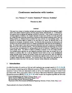
Figure 2. Geometry and inlet conditions for flow past a square-based prism. The coordinate system is indicated, and the distances are in units of the square height h 5 4 cm. The dotted lines indicate the lines along which the velocity profiles are measured. III. EXAMPLES: FLOW AROUND A SQUARE PRISM The flow around bluff bodies usually produces strong vortices in the wake, which in turn generate intense fluctuating forces on the body. The prediction of these forces is important in many applications. Such flows may involve complex phenomena such as unsteady separation and reattachment, vortex shedding and bimodal behavior, laminar subregions and transition to turbulence, high turbulence, and coherent structures, as well as curved shear layers. Recently such flows have received increasing attention, motivated in part by the engineering demand for accurate predictions but also by the desire to increase understanding of the underlying physical processes governing these flows. A square prism, mounted in a rectilinear channel, is chosen as a simple, representative bluff body, the separation points of which are fixed and known, unlike the case of a cylinder, where the separation points oscillate at the shedding frequency. The flow around and behind the prism is not only temporally but also spatially complex, with direct interaction between the separated shear layers and regions of irrotational flow entrained into the wake, requiring high local resolution. The flow configuration is presented in Fig. 2 and has a cross section of 10h314h, and a length of 20h where the prism has cross section h3h. The Re number based on h and the inlet velocity v ` is 21,400. Experimental profiles of the first- and second-order statistical moments of the velocity are available from Lyn et al.33 (Re521,400) and from Durao et al.,34 (Re514,800) at x 1 /h51 and 2 and on the center line ~the positions shown in Fig. 2!. Since all quantities are nondimensionalized with h and v ` , experimental ¯ and v rms from these experiments should be profiles of U ¯ 5 v x,` and able to be compared directly. At the inlet, U ¹ ¯p ex 50, where ex is the unit normal vector in the x x di¯ ex 50. For RAS, addirection; at the outlet, ¯p 5 p ` and ¹U tional boundary conditions have to be prescribed for k and e. The RAS calculations are two-dimensional, whereas the
Figure 4. Visualization of SGS kinetic energy (top) and enstrophy 21 ~ ¹ ¯ ! 2 , (bottom) behind a square prism. The calculation was performed 3U using the one-equation eddy viscosity LES model.
Figure 3. Comparison between velocity components for the experiment (symbols) and for calculations (profiles) using standard k 2 e , RNG k 2 e , Reynolds stress [using a model of Launder and Gibson (Ref. 35)], and LES using the Smagorinsky and one-equation eddy-viscosity models. The top diagram shows the U (streamwise) component of the velocity along the center of the domain. The next two figures show the U (left) and V (transverse, right) velocity components on a transverse plane at x/h 5 1, that is, one obstacle height downstream from the obstacle. The bottom two figures show the same profiles at x/h 5 2.
LES are three-dimensional, and thus a semiartificial free¯ ex 50 and (¹U ¯ ek )ek 50, k5y, z, is apslip condition, U plied on the planes xI e3 50 and 4h. For the top and bottom boundaries, x/h567h, slip conditions are applied while no-slip conditions are used for the boundary condition on the prism. The computational domain is discretized using a 250,000-cell grid. Results are shown in Fig. 3 from LES using the Smagorinsky27 and one-equation eddy-viscosity29 models, from RS using the Launder–Gibson Reynolds stress model,35 and the standard and RNG36 k2 e models. The function of the comparison is to illustrate the flexibility of FOAM for model implementation rather than to analyze the merits of the various models; a detailed analysis of the models will be described elsewhere. Hence, only a representative set of results is presented, these being the timeaveraged velocities U ~streamwise, that is, along the x axis! and V ~in the y direction!. There is a significant and unexplained discrepancy between the Lyn and Durao data for the U component on the center line, with the Lyn data
failing to show the expected return to the inlet velocity at large distances from the obstacle. The simple k2 e model performs poorly in this case, a result that has also been noted elsewhere. The other models all perform well, with the one-equation eddy-viscosity model and the LRR models predicting the near obstacle flow well. The accuracy of all models in capturing the recirculation behind the obstacle can also be enhanced by increasing the degree of refinement in this area. Further downstream all three models approach the data of Durao et al. The other results shown are the U and V components in the y direction at x/h51,2. Only the top half of the data is shown. The inadequacy of the k2 e model is clear. All the other models provide good predictions for the U component, with the main difference between the LES and RS models being the lack of smoothness in the curves, which is probably due to inadequate temporal averaging. The V component shows much larger discrepancies between the models, with the LES models outperforming the RS model at x/h51. Further downstream no model performs well. Overall, the LRR model produces results that are very similar to those of the LES models; however, this is not the case for more complex geometries. Figure 4 shows a perspective view of the flow around and behind the prism at one instant in time selected randomly from a LES with the one-equation eddy-viscosity model. The top part of Fig. 4 shows an isosurface of subgrid-scale turbulent kinetic energy k, and the bottom an ¯ ) 2 # . The gridisosurface of grid-scale enstrophy @ 21 (¹3U scale enstrophy traces the presence of the primary spanwise vortices, which are generated by Kelvin–Helmholtz instabilities in the shear layers originating from the separation points at the upstream corners of the prism and shed from COMPUTERS IN PHYSICS, VOL. 12, NO. 6, NOV/DEC 1998
627
alternate sides of the prism. It also traces the secondary streamwise vortices that envelop the primary vortices. k traces the subgrid-scale turbulence that arises from the breakdown of these vortices and correlates well with the vortex distribution. IV. OTHER EXAMPLES A. Stress analysis The traditional approach to solid-body stress analysis is using the FEM. However, the governing equations for fluid flow and for solid-body stress analysis are of a similar form, indicating that the FVM is also applicable as was demonstrated by Demirdzˇic´ and Muzaferija.37,38 This is not just a tour de force: problems involving solidification of a fluid ~welding or casting, for example! are most easily
solved if the same solution technique can be utilized in both phases. To demonstrate the ease with which FOAM can be used to develop a structures code, such a code will be presented, together with the simple example of the stress pattern generated by a circular hole in a rectangular plate. The plate material is assumed to be linear, elastic, and isothermal, and the assumption of infinitesimal deformation is made. Under these circumstances the displacement D can be solved for as a dependent quantity without introducing the complexity of how this affects the mesh. The time-dependent equation for the displacement D is
] 2D 5¹–@ m ~ ¹D1¹DT ! 1lI tr~ ¹D!# , ]t2
~12!
the FOAM representation of which is
for(runTime11; !runTime.end( ); runTime11) $ for(int iCorr 5 0; iCorr,nCorr; iCorr11) $ volTensorField gradU 5 fvc::grad(U); solve ( fvm::d2dt2(U) 55 fvm::laplacian(2*mu 1 lambda, U) 1 fvc::div ( mu*gradU.T( ) 2 (mu 1 lambda)*gradU 1 lambda*I*tr(gradU) ) ); % %
Note the split into implicit fvm and explicit fvc parts. This particular rearrangement guarantees diagonal dominance of the matrix and good convergence behavior. Iteration over the equation is required every time step for transient calculation in order to converge over the explicit contribution. For steady-state calculation, the inner iteration is unnecessary. Figure 5 shows the computational domain for the calculation of the stress field in a 2-D square plate with a circular hole in it. The plate is being stretched in one direction by uniform traction of 104 Pa. This is a relatively small load, and so the problem can be considered isothermal, linear, elastic, and steady-state. Since the plate is twodimensional, the assumption of plane stress is made. The hole is central to the plate, and so only one quarter of the domain need be simulated, symmetry boundaries being applied on the left and bottom. The mesh for this calculation contained 15,000 cells. The top boundary, together with the hole, are given zero-traction boundary conditions, while the right boundary has fixed traction of 104 Pa. The results are shown in Fig. 6 in the form of contours of s xx , s xy , and s y y . Apart from a small region in the plate’s center, the agreement is close. The error is in the region where several 628
COMPUTERS IN PHYSICS, VOL. 12, NO. 6, NOV/DEC 1998
blocks of cells making up the mesh meet; this produces a suboptimal arrangement of cells. The error is probably a result of the nonorthogonality of the mesh in this region. The stress concentration around the hole is clearly visible. This comparison shows that the solution is qualitatively correct; to demonstrate its quantitative accuracy, the analytical solution on the edge of the hole can be compared with the values from the FOAM calculation on this boundary. The results are shown in Fig. 7 as a function of angle around the hole ~Q50° being the x direction, that of the imposed strain!. The accuracy achieved is very good, with the maximum error being less than 2%. B. Magnetohydrodynamics calculation The flow of an incompressible conducting fluid with constant properties in a magnetic field is governed by the Navier–Stokes equations ¹–U50 ~13! ]U 1 1 1¹–~ U ^ U! 2¹–n ¹U52 ¹p1 J3B, ]t r r together with Maxwell’s equations,
Figure 5. Geometry of the domain for stress calculation. The various boundary types are indicated. In theory the domain should be infinite, in practice a domain 16 m on each side seemed to be adequate.
¹3H5J1
]D , ]t
¹–B50,
¹3E52
]B , ]t ~14!
¹–J50,
and Ohm’s law J5 s (E1U3B). To conform to accepted practice in electrodynamics, B is the magnetic field (B 5 m H) and D the electric displacement vector. Assuming that ] D/ ] t is negligible, then B2 1 1 B¹B, J3B5 ~ ¹3H! 3B52¹ 2m m and so the momentum equation takes the form
S
]U 1 B2 1¹–~ U ^ U! 2¹–n ¹U52 ¹ p1 ]t r 2m 1
~15!
D
1 ¹–~ B ^ B! . rm
~16!
Also, ¹3H5J5 s ~ E1U3B! ,
~17!
Figure 7. Variation of stress with angle around the hole. Curves are calculated from the analytical solution, while the symbols represent profiles extracted from the boundary field of the FOAM computation. Q 5 90° is the x direction (the direction of applied strain).
1 ]B 1¹–~ U ^ B2B ^ U! 2¹– ¹B50. ]t sm
~18!
These two transport equations for the system are in a form that can be solved using FOAM. The pressure equation is constructed from the total pressure ~static pressure p plus the magnetic pressure B 2 /2m !. A fictitious magnetic-flux pressure p H is introduced into the magnetic-field equation to facilitate the obeyance of the divergence-free constraint on B in the same manner as the pressure equation is used in PISO. The resulting field p H has no physical meaning, and at convergence represents the discretization error. A simple magnetohydrodynamics ~MHD! test case is the flow of an electrically conducting incompressible fluid between parallel insulating plates with an applied transverse magnetic field. Figure 8 shows such an arrangement, known as the Hartmann problem. The analytical solution for the velocity and magnetic field profiles are
and taking the curl results in
Figure 6. Comparison of calculated (top) and analytical (bottom) stress components for a square plate with a circular hole. From left to right: s xx , s xy , and s yy .
Figure 8. Geometry and symbol definition for the Hartmann problem. COMPUTERS IN PHYSICS, VOL. 12, NO. 6, NOV/DEC 1998
629
Figure 9. Comparison between computed profiles (symbols) and analytical profiles (solid lines) for MHD flow in a channel at Hartmann numbers M 5 1, 5, and 20. Shown on the left is the normalized velocity as a function of distance across the duct, and on the right is the nondimensionalized magnetic field component parallel to the flow. U cosh~ y 0 / d ! 2cosh~ y/ d ! , 5 cosh~ y 0 / d ! 21 v0 B v 0 m Asnr
52
S
D
~ y/y 0 ! sinh~ y 0 / d ! 2sinh~ y/ d ! , cosh~ y 0 / d ! 21
d5
1 B0
A
~19!
rn , s
where M 5y 0 / d is the Hartmann number. Figure 9 shows the analytical profiles of U and B compared with a calculation on a 4000-cell mesh. For M 51 the computed results are exact, which is not too surprising, since the profile is quadratic and FOAM uses second-order numerics by default. As the Hartmann number increases, the profiles become steeper, with greater curvature towards the edge of the duct. The error increases somewhat, although increased mesh resolution ~for example, a refined mesh towards the wall! will reduce this error. V. CONCLUSIONS As a discipline, CCM involves a wide range of issues: the physics of continua, the mathematical issues of manipulating the governing equations into a form capable of solution ~for example, the derivation of the LES and RAS equations for the mean flow!, the mathematical and physical issues of modeling terms in these equations, and the numerical and algorithmic issues of constructing efficient matrix inversion routines and accurate differencing schemes for the various derivatives. In a traditional, procedural approach to coding, the modeled equations have to be discretized and then written out in terms of components before coding can really begin. Since a typical general-purpose CFD code will be ;100,000 lines of code, the implementation of this is very challenging. The aim of this work was to produce a C11 class library ~FOAM! with which it is easy to develop CCM codes to investigate modeling and simulation of fluid flows. 630
COMPUTERS IN PHYSICS, VOL. 12, NO. 6, NOV/DEC 1998
In essence, FOAM is a high-level language, a CCM metalanguage, that closely parallels the mathematical description of continuum mechanics. As well as simplifying the implementation of new models, this makes checking the modeling more straightforward. This aspect is enhanced by the inclusion of features such as automatic dimension checking of operations. In addition to this, use of OOP methodology has enabled the dissociation of different levels of the code, thus minimizing unwanted interaction, and permitting research into the numerics ~differencing schemes and matrix-inversion techniques! to be largely divorced from that of modeling. A number of key properties of OOP that have enabled the development of FOAM are the following. ~1! The use of data encapsulation and data hiding enables lower-level details of the code, such as the implementation of the basic tensorial classes, to be hidden from view at the higher levels. This enables a user to deal only with aspects of the code relevant to the level of coding that they are involved in; for example, a new SGS model can be implemented without the need to access ~or even know about! the details of how the components of a tensor are being stored. Since a tensor is not simply a group of components but is a mathematical object in its own right, this is also aesthetically pleasing. ~2! Operator overloading allows the syntax of the CCM metalanguage to closely resemble that of conventional mathematics. This enhances legibility at high levels in the code. Although this approach increases the number of copying operations somewhat and involves more temporary storage than would be the case for a more traditional code, this has not been found to be a critical cost, and is more than compensated for by the ease of use of the resulting code. ~3! Function overriding and the use of virtual class hierarchies enable new low-level algorithms to be included in a manner that can be entirely transparent at higher levels. For example, constructing and implementing new
differencing schemes are complicated tasks; once implemented, the differencing scheme should be available to all high-level codes. By implementing a common interface for all differencing schemes through function calls div, grad, curl, ddt, etc., this can be accomplished. ~4! Polymorphism can also be used to give a common structure to higher-level elements of the code. Hence, a common framework for all LES SGS models can be constructed in the form of a virtual base class, and specific SGS models can be derived from this. This provides a mechanism whereby parts of the code can be switched at run time; it also assists in partitioning the code into independent sections. By appropriate use of derivation, the implementation of the SGS models can be made to reflect their internal structure as well. ~5! The distinction between interface and implementation and the rigorous hiding of the implementation make it possible to replace whole sections of the low-level code if this should become necessary, without problems higher up. ~In particular, the implementation of parallelization via domain decomposition can be made transparent to the top level through our implementation of interprocessor boundaries. Because of this, all FOAM codes parallelize immediately.! ~6! Code reuse, which is a major feature of OOP, is highly achievable in FOAM, since all CFD codes share a number of common features: differencing schemes, solvers, tensor algebra, etc. In summary, the application of OOP techniques to CCM has resulted in a powerful and flexible code for investigating numerics, modeling, and flow physics. Interaction between these levels has been kept to a minimum, and this makes the code easy to extend and maintain. The FOAM project demonstrates that it is possible to implement a mathematically oriented CCM metalanguage and has demonstrated its benefits. ACKNOWLEDGMENTS The LES work used as an example in this article was supported by the EPSRC under Grants No. 43902 and K20910 and by European Gas Turbines. REFERENCES 1. C. A. J. Fletcher, Computational Techniques for Fluid Dynamics, Springer Series in Computational Physics Vols. I and II, 2nd ed. ~Springer, Berlin, 1991!. 2. J. H. Ferziger and M. Peric´, Computational Methods for Fluid Dynamics ~Springer, Berlin, 1996!. 3. H. K. Versteeg and W. Malalasekera, An Introduction to Computa-
4. 5. 6. 7. 8.
9. 10. 11. 12. 13. 14. 15. 16. 17. 18. 19. 20. 21. 22. 23. 24. 25. 26.
27. 28. 29. 30. 31. 32. 33. 34. 35. 36. 37. 38.
tional Fluid Dynamics: The Finite Volume Method ~Longman Scientific and Technical, 1995!. B. W. R. Forde, R. O. Foschi, and S. F. Stiemer, Comput. Struct. 34, 355 ~1990!. B. Stroustrup, Proceedings of the 1st European Software Festival, 1991. B. Stroustrup, The C11 Programming Language, 3rd ed. ~Addison– Wesley, Reading, MA, 1997!. B. Stroustrup, OOPS Messenger, 1995, an addendum to the OOPSLA ’95 Proceedings. J. R. Cary, S. G. Shasharina, J. C. Cummings, J. V. W. Reynders, and P. J. Hinker, Comput. Phys. Commun. ~submitted!; available at http:// jove.colorado.edu/ ˜ cary/CompCPP – F90SciOOP.html. Y. Dubois-Pe`lerin and Th. Zimmermann, Comput. Methods Appl. Mech. Eng. 108, 165 ~1993!. J-L. Liu, I.-J. Lin, M.-Z. Shih, R.-C. Chen, and M.-C. Hseih, Appl. Numer. Math. 21, 439 ~1996!. Th. Zimmermann, Y. Dubois-Pe`lerin, and P. Bomme, Comput. Methods Appl. Mech. Eng. 98, 291 ~1992!. L. Machiels and M. O. Deville, ACM Trans. Math. Softw. 23, 32 ~1997!. Th. Zimmermann and D. Eyheramendy, Comput. Methods Appl. Mech. Eng. 132, 259 ~1996!. D. Eyheramendy and Th. Zimmermann, Comput. Methods Appl. Mech. Eng. 132, 277 ~1996!. H. Jasak, Ph.D. thesis, Imperial College, 1996. O. Ubbink, Ph.D. thesis, Imperial College, 1997. C. Fureby, G. Tabor, H. Weller, and A. D. Gosman, Phys. Fluids 9, 1416 ~1997!. S. Meyer, Effective C11 ~Addison–Wesley, Reading, MA, 1992!. M. R. Hestens and E. L. Steifel, J. Res. 29, 409 ~1952!. D. A. H. Jacobs, Technical report, Central Electricity Research Laboratories, 1980. H. A. van der Vorst, SIAM J. Comput. 13, 631 ~1992!. R. I. Issa, J. Comput. Phys. 62, 40 ~1986!. R. I. Issa, A. D. Gosman, and A. P. Watkins, J. Comput. Phys. 62, 66 ~1986!. B. E. Launder and D. B. Spalding, Comput. Methods Appl. Mech. Eng. 3, 269 ~1974!. V. C. Patel, W. Rodi, and G. Scheuerer, AIAA J. 23, 1308 ~1985!. B. E. Launder, G. J. Reece, and W. Rodi, ‘‘Progress in the development of a Reynolds-stress Turbulence Closure,’’ J. Fluid Mech. 68, 537 ~1975!. J. Smagorinsky, Mon. Weather Rev. 91, 99 ~1963!. U. Schumann, J. Comput. Phys. 18, 376 ~1975!. A. Yoshizawa, Phys. Fluids A 29, 2152 ~1986!. J. W. Deardorff, Trans. ASME, Ser. I: J. Fluids Eng. 156, 55 ~1973!. J. Bardina, J. H. Ferziger, and W. C. Reynolds, Technical Report No. TF-19, Stanford University, 1983. G. Erlebacher, M. Y. Hussaini, C. G. Speziale, and T. A. Zang, J. Fluid Mech. 238, 155 ~1992!. D. Lyn, S. Einav, W. Rodi, and J. Park, Technical report, Karlsruhe University, 1994. D. F. G. Durao, M. V. Heitor, and J. C. F. Pereira, Exp. Fluids 6, 298 ~1988!. M. M. Gibson and B. E. Launder, J. Fluid Mech. 86, 491 ~1978!. V. Yakhot, S. A. Orszag, S. Thangam, T. B. Gatski, and C. G. Speziale, Phys. Fluids A 4, 1510 ~1992!. I. Demirdzˇic´ and S. Muzaferija, Int. J. Numer. Methods Eng. 37, 3751 ~1994!. I. Demirdzˇic´ and S. Muzaferija, Comput. Methods Appl. Mech. Eng. 125, 235 ~1995!.
COMPUTERS IN PHYSICS, VOL. 12, NO. 6, NOV/DEC 1998
631