Replace this file with prentcsmacro.sty for your meeting, or with entcsmacro.sty for your meeting. Both can be found at the ENTCS Macro Home Page.
A Term Rewriting Technique for Decision Graphs Bahareh Badban1 Department of Software Engineering University of Konstanz Germany
Abstract We provide an automatic verification for a fragment of FOL quantifier-free logic with zero, successor and equality. We use BDD representation of such formulas and to verify them, we first introduce a (complete) term rewrite system to generate an equivalent Ordered (0, S, =)-BDD from any given (0, S, =)-BDD. Having the ordered representation of the BDDs, one can verify the original formula in constant time. Then, to have this transformation automatically, we provide an algorithm which will do the whole process. Keywords: Term Rewrite System; First-Order Logic; Decision Procedure; Verification
1
Introduction
In this article we consider the satisfiability and tautology problem for boolean combinations over the equational theory of zero and successor in the natural numbers. The atoms are equations between terms built from variables, zero (0) and successor (S). Formulas are built from atoms by means of negation (¬) and conjunction (∧). The formulas are quantifier-free, except for the implicit outermost quantifier (∀ when considering tautology checking, and ∃ when considering satisfiability). In general, the decision problem for plain equational theories is unsolvable already, so we must restrict to particular theories. The decision problem for boolean combinations over equational theories can be approached in several ways. Binary Decision Diagrams (BDDs) represent boolean functions as directed acyclic graphs [5]. They are of value for validating formulas in propositional logic. In [5] OBDDs (Ordered BDDs) are reduced BDDs which accept some ordering on boolean variables. A boolean function is satisfiable if and only if its unique OBDD representation does not correspond to 0. In the BDD-method, a formula is transformed to a propositionally equivalent Ordered Binary Decision Diagram (OBDD) which can be seen as a large if-then-else (ITE) tree with shared subterms (see Section 2). 1
Email:
[email protected] c 2009
Published by Elsevier Science B. V.
B. BADBAN
Although in principle also OBDD representations are exponentially big, it appears that in practice many formulas have a succinct OBDD-representation. Furthermore, boolean operations, such as negation and conjunction, can be computed on OBDDs very cheaply. Together with the fact that (due to sharing) many practical boolean functions have a small OBDD representation, OBDDs are very popular in verification of hardware design, and play a major role in symbolic model checking. In order to solve the satisfiability or tautology problem, each path in the OBDD has to be checked for consistency, with respect to the underlying equational theory. A path represents a conjunction of (negated) equations, on which the aforementioned decision procedures can be applied. All inconsistent paths can be removed, resulting in an OBDD with only consistent paths. However, due to sharing subterms, an OBDD can have exponentially many paths, so still there is a computational bottleneck. In the Encoding method these steps are reversed. First the formula is transformed to a purely propositional formula. In this translation, facts from the equational theory (e.g. congruence of functions, transitivity of equality and orderings) are encoded into the formula. Then a finite model property is used to obtain a finite upperbound on the cardinality of the model. Finally, variables that range over a set of size n are encoded by log(n) propositional variables. The resulting formula can be checked for satisfiability with any existing SAT-technique, for instance based on resolution [7] or on BDDs [5]. An early example is Ackermann’s reduction [1], by which second order variables can be eliminated. More optimal versions are in [10,17,6]. To date, several methods have been proposed to reduce different logics into propositional logic, which captures boolean functions. Goel et al. [10] and Bryant et al. [6]. present methods to transform the logic of Equality with Uninterpreted Functions (EUF) into propositional logic. In [18] the theory of separation predicates is reduced to propositional logic. In [16] the EUF extended with constrained lambda expressions, ordering, and successor and predecessor functions, is translated to propositional logic. The idea of extending the theory of BDDs was recognized earlier by Groote and van de Pol [11], who presented an algorithm to transform EQ-BDDs to EQ-OBDDs, where EQ-BDDs represent the extension of BDDs with equalities. We extend the method for EQ-BDDs from [11] to a fragment of quantifier free logic FOL. We make a terminating set of rewrite rules on (0, S, =)-BDDs, resulting in a (0, S, =)-R-OBDD, such that all paths in the (0, S, =)-R-OBDD are satisfiable. This property enables us to check tautology, contradiction and satisfiability on (0, S, =)-R-OBDDs in constant time. At the end we present an algorithm through which any formula of the logic above is translated to an (0, S, =)-R-OBDD. We define the set of terms as the closure of V¯ = V ∪ {0} (union of the sets of variables and zero) under successor. To be able to have an ordering on BDDs, we will need to define an ordering on terms of the logic. What is the appropriate ordering on terms? The answer, unfortunately, is not obvious. In [2] Chapter 3, two orderings which resulted in failed attempts are explained. One of them does not provide termination, and the other does not omit all unsatisfiable paths. The approach introduced here is in a sence a variant of [3], though our new ordering yields some simpler representation of the terms in the proof settings. Besides, it provides an alternative technique for the OBDD transformation. This, as 2
B. BADBAN
p
⊤
q
⊤
⊥
Figure 1. ITE (p, ⊤, ITE (q, ⊤, ⊥)). Solid lines denote the left branch of the ITE (when their corresponding guard holds) and dashed lines represents their counterpart.
a result can offer a different method for possible extensions of the background logic (notice that as mentioned above, finding the right order is not easy, and this problem would remain for bigger theories as well). In the current work, substitution rules are certainly different than those of the previous work. In addition, we also introduce an automatic way for transforming any formula (in our FOL fragment) into some Ordered BDD. We do this by means of a so called sort algorithm. Road map. In Section 2, we describe BDDs, and give a formal syntax and semantics of (0, S, =)-BDDs. In Section 3 our transformation is presented, leading to the set of (0, S, =)-R-OBDDs. First a total and well-founded order on variables is assumed, and extended to a total well-founded order on equalities. Then the rewrite system is presented. Finally, we prove termination and satisfiability over all paths. Section 4 presents an algorithm with the same result as the given term rewrite system. Finally, Section 5 concludes with some remarks on implementation and possible applications.
2
Binary Decision Diagrams
A binary decision diagram [5] (BDD) represents a boolean function as a finite, rooted, binary, ordered, directed acyclic graph. The leaves of this graph are labeled ⊥ and ⊤, and all internal nodes are labeled with boolean variables. A node with label p, left child L and right child R, written IT E(p, L, R), represents the formula if p then L else R. Given a fixed total order on the propositional variables, a BDD can be transformed to an Ordered binary decision diagram (OBDD), in which the propositions along all paths occur in increasing order, redundant tests (ITE (p, x, x)) don’t occur, and the graph is maximally shared. For a fixed order, each boolean function is represented by a unique reduced OBDD (in the sequel we simply use OBDD to denote a reduced OBDD). For more information on that, one can see [5]. Example 2.1 Figure 1 illustrates a BDD representation of the following formula: ITE (p, ⊤, ITE (q, ⊤, ⊥)) where p and q are propositional variables. 2.1
BDDs with Equality, Zero and Successor
In this section we introduce some basic notations and definitions. We also provide the syntax and semantics of BDDs extended with zero, successor and equality. For our purpose, the sharing information present in the graph is immaterial, so we 3
B. BADBAN
formalize BDDs by terms (i.e. trees). We show that every formula is representable as a BDD. We assume V is a set of variables, and define V¯ = V ∪ {0}. Sets of terms, formulas, guards and BDDs are defined below: Definition 2.2 Terms t ∈ W , formulas ϕ ∈ Φ, guards g ∈ G and (0, S, =)-BDDs T ∈ B are defined by the following grammar (with x ∈ V ): t ::= 0 | x | S(t) ϕ ::= ⊥ | ⊤ | t = t | ¬ϕ | ϕ ∧ ϕ | ITE (ϕ, ϕ, ϕ) g ::= ⊥ | ⊤ | t = t T ::= ⊥ | ⊤ | ITE (g, T, T ) A guard is trivial if it is ⊥ or ⊤, and otherwise it is non-trivial. Here are some notations that we will use in this paper: In order to avoid confusion with the =symbol in guards, we use ≡ to identify syntactic equality between terms or formulas. Symbols x, y, z, u, . . . denote variables; r, s, t, . . . range over W ; ϕ, ψ, . . . range over Φ; f, g, . . . range over guards. Var(t) represents the variable occurring in term t. Furthermore, we will write x 6= y instead of ¬(x = y) and S m (t) for the m-fold application of S to t, so S 0 (t) ≡ t and S m+1 (t) ≡ S(S m (t)). Note that each t ∈ W is of the form S m (u), for some m ∈ N and u ∈ V¯ . We will use some fixed interpretation for the above formulas: Terms are interpreted over the natural numbers (N) and for formulas we use the classical interpretation over {0, 1}. Given a valuation v : V → N, we extend v homomorphically to terms and formulas as: v(0) = 0 v(S(t)) = 1 + v(t) v(⊥) = 0 v(⊤) = 1 v(s = t) = 1, if v(s) = v(t), 0, otherwise. v(¬ϕ) = 1 − v(ϕ) v(ϕ ∧ ψ) = min(v(ϕ), v(ψ)) v(ITE (ϕ, ψ, χ)) = v(ψ) if v(ϕ) = 1, v(χ) otherwise. It is trivial that the value of a formula under any valuation function is either 0 or 1. Given a formula ϕ, we say it is satisfiable if there exists a valuation v : V → N such that v(ϕ) = 1; it is a contradiction otherwise. If for all v : V → N, v(ϕ) = 1, then ϕ is a tautology. Finally, if v(ϕ) = v(ψ) for all valuations v : V → N, then ϕ and ψ are called equivalent. v satisfies ϕ (or equivalently ϕ holds under v) is denoted as: v |= ϕ. 4
B. BADBAN
Lemma 2.3 Every formula in Φ is equivalent to at least one (0, S, =)-BDD.
Representant-Ordered (0, S, =)-BDDs
3
The first step to make a BDD ordered, is to simplify all its guards, in isolation. Here, simplification on guards will be done by Definition 3.2. In Section 3.1 we present a new order on terms. In Definition 3.8 we define an ordering on guards. Notice that these definitions are different from those of [3]. Thereafter, we will introduce a term rewrite system. Using this system we simplify BDDs to their most reduced form, denoted as (0, S, =)-R-OBDD. 3.1
Definition of (0, S, =)-R-OBDDs
We consider a fixed total and well-founded ordering on V . Below we assume that the variables x, y and z are ordered as x ≺ y ≺ z. Definition 3.1 [ordering definition] We extend ≺ to a total order on W : •
0 ≺ u for each element u of V
•
S m (x) ≺ S n (y) if and only if x ≺ y or (x ≡ y and m < n) for each two elements x, y ∈ V¯
As of now, we may use the term OBDD instead of (0, S, =)-R-OBDD, for simplicity. Definition 3.2 Suppose g is a guard. By g ↓ we mean the normal form of g obtained after applying the following rewrite rules on it: x=x → ⊤ S(x) = S(y) → x = y 0 = S(x) → ⊥ x = S m+1 (x) → ⊥
for all m ∈ N
t = r → r = t for all r, t ∈ W such that r ≺ t. We call g simplified if it cannot be further simplified, i.e. g ≡ g ↓. A (0, S, =)-BDD T is called simplified if all guards in it are simplified. Lemma 3.3 If g ∈ G is simplified to g′ using Definition 3.2, then g and g′ are equivalent. Next lemma shows possible shapes of a simplified guard. In contrast to [3] the smaller term sits on the left. Lemma 3.4 If g is a simplified guard, then it has one of the following shapes: •
S m (0) = x
• S m (x) •
=
for some x ∈ V
S n (y)
for some x, y ∈ V, x ≺ y, m = 0 or n = 0
⊤ or ⊥ 5
B. BADBAN
It is worth mentioning that as a result each guard has only one simplified form. In order to be able to substitute one term by another, we may often need to upraise the atom which includes the term by applying some few additional successors, and then to do the replacement. Below, we explain our strategy for doing this: Definition 3.5 Let m ∈ N. For terms r, t ∈ W , a variable y ∈ V and a guard g ∈ G we define: (r = t)↑m := S m (r) = S m (t) (lifting) Definition 3.6 Suppose g is a simplified non-trivial guard, y ∈ V and t, r ∈ W . We define: ( (g↑m [S m (y) := r]) ↓ if y occurs in g g|r=S m (y) := g otherwise ( ⊥ if g ≡ (t = r) ↓ g|t6=r := g otherwise The following lemma shows the soundness of the operations above: Lemma 3.7 For any guard g and a positive natural number m, g ↑m and g are equivalent terms. Moreover, for a guard f , if v |= f for some valuation v then v(g) = v(g|f ). To have ordered BDDs, we need to impose some order on simplified guards. Below is what we use as the ultimate order on such guards: Definition 3.8 [order] We define a total order ≺ on simplified guards as: •
⊥ ≺ ⊤ ≺ g, for all simplified guards g different from ⊤, ⊥.
•
(S p (x) = S q (y)) ≺ (S m (u) = S n (v)) iff: i) ii) iii) iv)
x ≺ u or x ≡ u, p < m or x ≡ u, p ≡ m , y ≺ v or x ≡ u, p ≡ m, y ≡ v, q < n
According to this definition (r1 = t1 ) ≺ (r2 = t2 ) iff (r1 , t1 ) ≺lex (r2 , t2 ), in which ≺lex is a lexicographic order on quadruples of the total, well-founded orders (V¯ , ≺) × (N,