Please do not quote without the authors’ consent.
A Theoretical Framework to Evaluate Different Margin-Setting Methodologies: with an Application to Hang Seng Index Futures a
Chor-yiu SIN * Kin LAM c Rico LEUNG b
a
Hong Kong Baptist University, Department of Economics, School of Business, Waterloo Road, Kowloon Tong, Hong Kong, Tel: (852) 3411 5200, Fax: (852) 3411 5580, e-mail:
[email protected] b Hong Kong Baptist University, Department of Finance and Decision Sciences, School of Business, Waterloo Road, Kowloon Tong, Hong Kong, Tel: (852) 3411 5007, Fax: (852) 3411 5585, e-mail:
[email protected] c Securities and Futures Commission, Supervision of Markets Division, 12th Floor, Edinburgh Tower, The Landmark, 15 Queen’s Road Central, Hong Kong. Tel: (852) 2840 9357 Fax: (852) 2521 7917, e-mail:
[email protected] (The view expressed in this paper does not represent any view of the Securities and Futures Commission) * Corresponding author
This version: December 14, 2002
Abstract The margin system is a clearinghouse’s first line of defense against the default risk. From the perspectives of a clearinghouse, the utmost concern is to have a prudential system to control the default exposure. Once the level of prudentiality is set, the next concern is the opportunity cost to the investors. It is because high opportunity cost discourages people from hedging futures and thus defeats the function of a futures market. In this paper, we first develop different measures of prudentiality and opportunity cost. We then formulate a statistical framework to evaluate different margin-setting methodologies, all of which strike a balance between prudentiality and opportunity cost. Four margin-setting methodologies, namely, one using simple moving averages, one using exponentially weighted moving averages, one using a GARCH-GJR approach, and the last one using the lagged implied volatility (whenever it is available), are applied to Hang Seng Index Futures. The lagged implied volatility by and large has the best performance, while the GARCH-GJR approach is a best substitute when implied volatility is not available. JEL Classification: G14, G15 Keyword(s): Expected shortfall, implied volatility, margin-setting methodologies, opportunity cost, prudentiality, value-at-risk
1
1. Introduction
In all financial markets, the institutions responsible for clearing and settlement are the exchange and the clearinghouse, particularly the latter. Bernanke (1990) points out that in some cases, the clearinghouse is a part of the exchange; otherwise, it is a separate nonprofit corporation. That said, all clearinghouses also function as an association of the clearing members. Being members of the clearinghouse, private firms acquire the right to clear trades of their own customers and for non-member firms.
Apart from these,
clearing members can also do proprietary trading and clear trades of their own. Consequently, a clearing member may end up with a net position in futures trading. The clearinghouse stands in the center of the settlement process, disbursing payment and receiving payments to and from clearing members. Thus a clearinghouse provides a central counter-party function that assumes the default risk of its clearing members. This setup greatly reduces the members’ counter-party risk as the clearinghouse now acts as a counter-party to all members and the clearinghouse is well known to be very prudent in risk management and is backed up by a substantial amount of reserve funds.
Being a central counter-party, a clearinghouse normally bears no market risk since at all times, the market values of the long and the short position cancel each other out. However, a clearinghouse is exposed to the its members’ default risk. When a clearing member defaults, the clearinghouse needs to liquidate the member’s position. A clearing member defaults because its clients do, or because the loss in its own proprietary account forces it to do so. In view of the members’ default risk, a clearinghouse may adopt various measures. It may require a member to have a minimum capital requirement, to 2
pay up a guarantee fund, or to report on firm capital regularly, to name just a few. Among all the risk management measures, the most important one is to put up an initial/maintenance margin money and to require that its members do likewise for their clients. The initial/maintenance margin is set at a multiple of a member’s net position or its gross position, though most clearinghouses in the world charge margins on a net basis. That is, when the margin money is not sufficient to cover the loss of a member at market close, the member is asked to mark its position to market. Default occurs if the member fails to comply and the clearinghouse has to liquidate the member’s assets to cover the losses. If that is still not sufficient, the reserve fund is dipped into to cover the shortfall.
While it is advisable to have a low default probability, one minuses which is called coverage probability throughout this paper, setting it too low ends up with a very high margin level. Booth, Broussard, Martikainen and Puttonen (1997) point to the simple dilemma faced by a clearinghouse. If the margin level is set too low, the margin money may not be large enough to cover the losses. On the other hand, if the margin level is set too high, all members suffer from large opportunity cost in hedging with futures. In a policy paper, Baer, France and Moser (1994) are the first ones who advocate that any margin setting is supposed to take into account the opportunity cost of margin deposits. This consideration turns out to be the kernel of various issues tackled in this paper.
This paper is organized as follows. In Section 2, we start with the background of this study, which consists of a brief literature review and a description of the possibly different roles played by a clearinghouse. In Section 3, we formally propose a theoretical framework, which can be used to compare various margin-setting methodologies. In 3
particular we propose some quantitative measures of prudentiality and opportunity cost. In Section 4, we describe how margin levels are usually determined by a benchmark formula driven by volatility estimates, which are often the major focus of practitioners as well as academics who work on financial econometrics. In particular, the prototypes of four methodologies will be discussed: (1) the historical volatility model using simple moving averages, (2) the model using exponentially weighted moving averages, (3) the GARCH model, and (4) the model using lagged implied volatility (when the options of the underlying asset is traded). Using the theoretical framework proposed in Section 3, as an illustration, the four methodologies are compared with the Hang Seng Index (HSI) futures data. Section 5 contains the empirical results with the full sample while Section 6 presents the further empirical results with the sub-sample that covers the period within which the implied volatility is available. Section 7 concludes the paper.
2. Background of this study
Admittedly, the initial/maintenance margin is the first line of defense for a clearinghouse to guard against its members’ default risk. Setting the margin at the right level is of paramount importance and it has been an interesting topic to numerous financial scholars. In the literature, prudential margin setting is often recommended and the main objective is to control margin level prudentially such that the default probability is acceptable to the clearinghouse. For instance, Duffie (1989) points to the fact that a clearinghouse often uses statistical theories to determine the margin level to guard against defaults. Figlewski (1984) suggests a methodology for analyzing the degree of protection 4
afforded by different margin levels based on the computation of a “first passage time” probability distribution. Gay, Hunter and Kolb (1986) derive the probability of a margin violation on a given date for a given margin level. They argue that margins on different commodities contracts should be set such that the probability of the futures price moving by an amount equal to or greater than the margin during a given time interval was constant across contracts. Warshawsky (1989) shows that the normality assumption is inappropriate and thus the margin level is often underestimated. Fenn and Kupiec (1993) develop alternative models of an efficient prudential margin management policy using the paradigm of efficient contract design proposed by Brennan (1986). Recently, a number of authors used extreme value theory to determine the appropriate margin levels. See for instance Longin (1999,2000), and Cotter (2001). In all these papers, the main concern is a margin level prudential enough to guarantee a small default probability though it is difficult to spell out exactly how small it should be.
There is no doubt that the way to evaluate a margin-setting methodology depends on the role(s) played by a clearinghouse. Baer et al. (1994) argues, among many other things, that when a clearinghouse is treated as a club, it should set the margin at a level that benefits all its members. Should it be the case, the opportunity cost of margin money as well as the members’ loss (when there is a default) can be pooled together and the margin level should be set to minimize the (expected) total cost. For sake of exposition, we call this a model of “clearing members”.
In sum, in a market where the clearinghouse is a club of its members, it is right to say that a clearinghouse’s primary concern is the members’ interest and thus the “clearing 5
members” model applies. However, in recent years, some exchanges were demutualized and they become listed companies owned by non-user shareholders. Examples include the Australian Stock Exchange, the Hong Kong Exchanges and Clearing Limited (HKEx), and the Singapore Exchange. As a listed company, the ownership structure dictates and a clearinghouse takes care of its shareholders’ interest and thus a profit maximization approach is adopted. Under such a model, margin should be set at a level so as to maximize the exchange’s overall profit.
Similarly, we call this a model of “listed
company”.
Nevertheless, neither model discussed above is applicable when a clearinghouse also has a public role, as there are conflicts between public responsibility of a clearinghouse and its business concerns. For the interest of the public, clearinghouses in some countries of the world are obliged by law to ensure a sound and safe risk management system, so as to maintain the integrity of the local financial system. Take Hong Kong as an example. Clearing is now done through the Hong Kong Exchanges and Clearing Limited (HKEx). 1 This merged entity is an independent body detached from the firms that have trading rights and/or clearing functions. Since the merge in Year 2000, the HKEx has become a listed company possibly owned by the non-user shareholders. On the other hand, the public interests are protected by the Exchanges and Clearing Houses (Merger) Ordinance (Caption 555). The ordinance requires the HKEx to maintain an orderly and fair market and to manage risks prudently. Moreover, in the event that the public interests conflict with any other interests which HKEx is required to serve under 1
The Stock Exchange of Hong Kong Limited, Hong Kong Futures Exchange Limited, and Hong Kong Securities Clearing Company Limited used to be three separate entities. In Year 2000, they are merged
6
any other law, the public interests prevail. Under this arrangement, the clearinghouse in Hong Kong can hardly be a club of clearing members nor a purely profit-maximizing listed company. This situation is not unique and quite a number of clearinghouses in the Asian area assume a public role of maintaining market integrity.
For these
clearinghouses it seems that the higher the margin the better is the protection. Nevertheless, it is not in the public interest if too high a margin is charged to investors, as the market liquidity is affected. In this regard, Figlewski (1984) notes that a liquid futures or options market is in the public interest, and that it would be counter-productive to impose too high a margin on investors as market liquidity will decrease. Hence, considerations should also be given to the investors’ opportunity costs. All in all, how to strike the balance between prudentiality and opportunity cost without actually merging them into one term is definitely an important issue, which in turn is the main focus of this paper.
In our approach, prudential concern is of primary importance and secondary concern will be given to opportunity cost consideration. Our approach differs from those in many other papers that simply consider prudential concerns and leave opportunity cost unattended. Our approach also differs from those in other papers in which prudential concerns and opportunity cost are treated in parallel. We can draw an analogy of our approach to that in the statistical testing of hypothesis. In statistical hypothesis testing, the control of a type I error is of primary concern. Once the type I error is controlled, attention is paid to control also the type II error. Having a margin level not large enough to cover a loss is here treated as a type I error and opportunity cost is treated as a type II
under a demutualization act that was in turn put forth by the Hong Kong Special Administrative Region
7
error.
Just as we can compare two statistical tests with the same probability of
committing a type I error, we can compare two margin-setting methodologies with the same prudential level. In the former, we compare their probabilities of committing a type two II error and in the latter, we compare their opportunity costs.
It is worth-mentioning that our paper contrasts vividly with the existing literature that relates the margin requirements with volatility. See, for instance, Hardouvelis (1990), Hardouvelis and Peristiani (1992) and Hardouvelis and Kim (1995). (See also Hsieh and Miller, 1990, who obtain some opposite results.) Among many other things, the literature investigates the causal relationships from margin requirements to volatility; while as one can see in the following sections, our margin requirements are based on different models of exogenously given volatility.
We close this section with a paragraph on the development of the margin-setting system in the HSI futures market, which is the focus of the empirical part of this paper. About one year after it started to be traded, following three successive day’s decline on the U.S. stock market, the stock market in Hong Kong fell by about 11.1% on October 19, 1987. The clearinghouse then, ICCH (Hong Kong) Limited, made an intra-day margin call at midday on all members holding long positions in the HSI futures contract to collect an additional margin of HK$8,000 per contract. The margin level was further increased to $10,000 per contract at 3:00pm of the same day. On the next day, the Stock Exchange of Hong Kong decided to suspend trading in the stock market for four days. Following this decision, the Hong Kong Futures Exchange also suspended trading of the
Government.
8
HSI futures contract for four days. Later on the same day, some futures brokers had difficulties in collecting margins from their clients. The Hong Kong Futures Exchange pointed out that there were serious doubts about the ability of the Hong Kong Futures Guarantee Corporation, which had a capital of HK$15 million and accumulated reserves of around HK$7.5 million, to meet its obligations as a result of huge amount of default. As the futures market could not resume trading without some reinstatement of the guarantee, the Government, Hong Kong Futures Exchange and various market participants met to discuss how to resolve the problem. A support package was put together over the weekend of October 24-25. The package was a loan of HK$2 billion to the Hong Kong Futures Guarantee Corporation comprising HK$0.5 billion from its shareholders, HK$0.5 billion from a number of the major brokers and HK$1 billion from the Government’s Exchange Fund. Repayment would be through a transaction levy on the futures market, a special levy on the stock market and from delayed payments by and recoveries from defaulting members. Both the stock and futures markets reopened at 11:00am, October 26. The stock market opened sharply lower and the HSI plunged 1,120 points to close at 2,242 points, representing a 33% fall. In the futures market, the spot month contract lost 1,544 points or 44%. The margin level of HSI futures contract was further increased from HK$10,000 to HK$25,000 per contract. Given this significant fall on that day, the initial support package might not provide the Hong Kong Futures Guarantee Corporation with sufficient financial resources to continue its operations. Arrangements were made in that evening to provide an additional HK$2 billion support facility (this facility expired on 26 April 1988 without having been drawn down). Finally, a total of HK$1.795 billion was drawn from the initial support facility to enable the Hong Kong Futures Guarantee to meet its obligations. After the October Crisis, the Hong Kong 9
Futures Exchange set up its own clearing house, HKFE Clearing Corporation, and revamped the risk management system. A Reserve Fund was established to replace the guarantee function provided by the Hong Kong Futures Guarantee Corporation. Margin levels were set and adjusted based on the market volatility.
2
3. A theoretical framework for comparing margin-setting methodologies
As we emphasized in Sections 1 and 2, margin-setting methodologies should be compared in terms of “prudentiality” and “opportunity cost” with the understanding that prudentiality concern is primary and opportunity concern is secondary. To achieve this aim, we need to construct a prudentiality index (PI) and an opportunity cost index (OCI), with the following properties:
1.
A higher PI means a higher level of prudentiality and is more preferable to a lower PI.
2.
A lower OCI means a lower opportunity cost and is more preferable to a higher OCI.
3.
With a long data history, PI and OCI can be estimated with high accuracy.
With these two indexes, we can now compare the performance of two marginsetting approaches A and B using a historical data set.
Suppose approach A is
parameterized by a parameter α (possibly a vector) and approach B is parameterized by a
2
This paragraph is excerpted from Davison (1988).
10
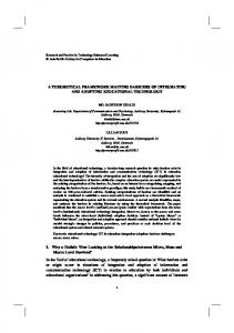
parameter β (also possibly a vector). For a given parameter α, A can be represented by a point in the “prudentiality-opportunity cost” space, say P in Figure 3.1 below. By varying the parameter α, A can be represented by a curve in the “prudentialityopportunity cost” space, as also shown in Figure 3.1. Note that the curve is upward sloping as higher prudentiality is obtained at the expense of opportunity cost.
Figure 3.1 is here
Similarly, B can be represented by another curve as also shown in Figure 3.1. Consider two points P and Q with the same prudentiality index PI0. The fact that point P is above point Q implies that A incurs a higher opportunity cost than B and hence B is preferred to A, when prudentiality index equals PI0. In Figure 3.1, B incurs a lower opportunity cost over A for all levels of prudentialilty. Thus, B is uniformly superior to A.
However, the comparison between A and B may not be uniform. An alternative possibility is shown in Figure 3.2.
Figure 3.2 is here
In Figure 3.2, B performs better than A if we are interested in prudentiality level beyond PI0, otherwise, A performs better. Should it be the case, the choice between A and B depends on the range of prudentiality index which the clearinghouse finds appropriate.
11
Prudentiality Index I: Coverage Probability (CP)
A common measure of “prudentiality” of a prescribed margin level is the coverage probability (CP), which is defined as the probability that the margin collected is sufficient to cover the losses arising from the actual price change in the market. The margin is usually set at a level so that CP is higher than 95%. For a more prudent approach, CP can be set as 98% or even higher than 98%.
Prudentiality Index II: Expected Shortfall (ESF)
Other than CP, there is another way to measure prudentiality with dollar value as a unit of measurement. Note that a prudential margin should have the following effect: margin money collected (M) is enough to cover the loss (L). The margin shortfall, which is defined as the loss beyond what could be covered by the margin money, should desirably be zero. Naturally, the expected shortfall (ESF) can be used to measure the degree of prudentiality. In other words, ESF can be expressed in terms of L and M as follows: ESF = E[(L-M)+],
0 L − M
where (L-M)+ =
if L ≤ M . if L > M .
Since a prudentiality index should have the property that higher is the index, higher is the prudentiality level, the negative value of ESF is used as a prudentiality index. In fact the ESF used here is similar to various measures of default exposure suggested in 12
the literature. See, for instance, Bates and Craine (1999). While Bates and Craine (1999) focus on valuing the default exposure (or “prudentiality “in our terminology), we use it to study the tradeoff between “prudentiality” and “opportunity cost”.
On the other hand,
the ESF has been found a better alternative to Value-at-Risk (VaR) in the literature of risk management. See, for instance, Acerbi and Tasche (2002) and Tasche (2002).
Opportunity Cost Index I: Expected Margin Level (EML)
We now turn to constructing an opportunity cost index. Baer et al. (1994) point out that an increase in margin level may drive up the marginal cost of funds and different investors may have different marginal costs. To simplify the situation, we assume here that the opportunity cost is on a per contract basis and is simply a constant multiple of the margin level. Thus the expected margin money per contract can be taken as a natural measure of opportunity cost. Even if the cost of money is not directly proportional to the size of the margin level, it must be true that a higher margin level will inflict a higher cost of funds. Thus, for comparative purposes, a comparison of margin levels should suffice.
Opportunity Cost Index II: Expected Overcharge (EOC)
Instead of using the margin level as a measure of opportunity cost, an alternative is to use the expected overcharge (EOC). In fact, from an investor’s viewpoint, paying a margin money M is seen to be excessive if the actual loss resulting from her/his position amounts to L which is smaller than M. Thus, EOC is a sensible measure of opportunity cost. Using the notation introduced above, 13
EOC = E[(M-L)+],
where (M-L)+ = M − L 0
if if
M ≥ L. M < L.
A remark on ESF and EOC is in order. It is not difficult to see that
EOC + ESF = E(|M-L|), EOC – ESF = E(M-L).
That is, neither the sum nor the difference of ESF and EOC is a constant. Instead, both the sum and the difference depend on the margin money M and the loss L, which in turn depend on the parameter(s) of the margin-setting methodology. In this sense, EOC adds a new dimension to ESF.
Let Pt and Rt be respectively the index futures price and the daily return rate for trading day t. Throughout this paper, all the margin-setting methodologies considered depend on the conditional mean and variance of the daily return rate, which are denoted as µt and σt respectively. Different indexes of prudentiality or opportunity cost can be estimated with historical data. CP is estimated by the empirical probability, denoted by ECP; while EML is estimated by the sample average of margin level, denoted by AML. In a similar token, ESF is estimated by the sample average of the daily shortfall SFt, where for each trading day t, 14
SFt ≡ 0,
≡ Pt-1(|Rt| - |µt + kσt|),
if |µt + kσt| ≥ |Rt|. if |µt + kσt| < |Rt|.
On the other hand, EOC is estimated by the sample average of the daily overcharge OCt, where for each trading day t,
OCt ≡ Pt-1( |µt + kσt| - |Rt|),
≡ 0,
if |µt + kσt| > |Rt|. if |µt + kσt| ≤ |Rt|.
4. Benchmark formulae for different margin-setting methodologies
It is commonly accepted that margin-setting should not rely on a mechanical formula. In determining an appropriate margin level, factors other than volatility need to be considered and margins are optimally set by a designated margin committee in a clearinghouse, as suggested by Brenner (1981). The committee has the discretion to change the margin level whenever it thinks fit for risk management purposes. However, it is not uncommon for clearinghouses in the world to use a formula-driven margin level as a reference level for margin. The formula is usually volatility driven and the margin so determined is called a benchmark margin.
There are many ways to estimate the conditional volatility and a benchmark formula may give rise to different margin levels depending on which volatility forecasts 15
are used by the clearinghouse. As far as we know, there exists no systematic way to decide whether one forecast is better than the other, or alternatively put, whether one margin setting methodology is superior to another. In Section 3 above, we offer a theoretical framework for evaluating methodologies for margin setting.
A benchmark formula usually relates the margin level to volatility. Margin is set at a level Pt-1|µt+kσt|, where Pt-1 is the futures price in the previous trading day, k is a prescribed constant, and µt and σt are respectively the mean forecast and the volatility forecast.
3
It should be emphasized that we do not assume that the normalized return
rate is normally distributed. In fact, by increasing k, we allow the return has a heavier tail. See the discussion on the empirical findings in Section 5.
Simple Moving Averages (SMA)
The simplest estimators for µt and σt are historical mean return and standard deviation of return. That is, given the returns Rt-1, Rt-2, …, Rt-T over a T-day historical period:
µt = σ t2 =
1 T ∑ Rt −i . T i =1 1 T ∑ ( Rt −i − µ t ) 2 . T − 1 i =1
16
For sake of exposition, we this approach is called “historical volatility” or “simple averages”. This approach involves two parameters: T and k. The parameter k has the obvious property that an increase in k will increase “prudentiality” but will induce a higher “opportunity cost”. However, the effects of T on “prudentiality” and “opportunity cost” are not that obvious. Various clearinghouses have different choices of T and k. Based on an internal report of the Hong Kong Futures Exchange published in 1998, we report the choices of T and k in various exchanges are summarized in Table 4.1 below. Note throughout the paper, we follow the common practice and present the margin level in index point.
4
Table 4.1 is here
Exponentially Weighted Moving Averages (EWMA)
One obvious shortcoming of the “historical volatility” approach is that volatility forecast places equal weight on all returns, recent or remote. Due to the widely accepted fact that volatilities are positively auto-correlated, a formula that places heavier weights on recent returns than on remote returns should give a more accurate forecast. In view of this, Hong Kong Futures Exchange (HKFE) used an exponentially weighted moving averages (EWMA) formula in its benchmark margin setting. See Lam, Lee, Cox, Leung
3
Unlike other papers such as Booth et al. (1997), same margin requirement is applied to both short and long position. This is a common practice for many, if not all, clearinghouses, as they are not supposed to take position on the markets. 4 Heuristically the futures price and thus the margin level follows a random walk with a positive drift. Hence our results may be dominated by the later part of the sample. We also repeat our empirical work with the margin level expressed in percentage of lagged futures price. The results obtained are qualitatively the same as those in Sections 5 and 6. Thus those results are not reported.
17
and Zhou (1999). While EWMA has long been used for mean forecast in the literature of time series analysis, recently it attracts a lot of attention under the topic of volatility forecast. 5 In an EWMA formula, margin is set at the level Pt-1|µt+kσt| where k is a constant and the mean µt and the volatility σt are updated by exponential smoothing as follows:
µt = λRt-1 + (1-λ)µt-1, σ t2 = λ(Rt-1 - µt-1)2 + (1-λ) σ t2−1 , where λ is a smoothing parameter.
Generalized Autoregressive Conditional Heteroskedasticity-GJR (GARCH)
The EWMA formula in turn suffers from its ad-hoc nature, as there is no theoretical justification of preferring one λ value to another. In this paper, we also consider a GARCH approach for volatility forecast, with the modification suggested by Glosten, Jagannathan and Runkle (1993) (henceforth GJR). An appropriately long time series of historical data is used to estimate the GARCH parameters. The GARCH model will then provide a forecast of the volatility σt, conditional upon the past volatilities. The margin level is then set as Pt-1|µt+kσt|, with µt and σt now being the conditional mean and the conditional standard deviation. In this model, we assume that the underlying return process follows a GARCH(1,1) process. At the end of trading day t-1, the GARCH(1,1) parameters are estimated using historical returns Rt-1, Rt-2, … , Rt-N, where N is a given constant. In other words, we use historical data of N days in forecasting the volatility in
5
A prominent example is RiskMetrics in which the EWMA volatility forecast is adopted in the Value-atRisk (VaR) measurement. See J.P. Morgan (1996).
18
day t. Notice that computational efforts are relatively high as estimation is done for every trading day. More precisely, the parameters are estimated with the following quasi-loglikelihood function:
( Rs − γ t ) 2 1 1 2 , ∑ l s , where ls = − ln(2π) − ln( σ s ,t ) − s =t − N 2σ s2,t 2 2 t −1
t
t
σ s2,t = α 0t + α 1t (Rt-1 - γt)2 + α 2t (Rt-1 - γt)2It-1 + α 3t σ s2−1,t , where the indicator function It-1 = 1 if Rt-1 - γt < 0. γ t , α 0t , α 1t , α 2t and α 3t are the model parameters at the end of day t-1. The term α 2t , which is first proposed in GJR, captures the potential asymmetric volatility response to negative and positive returns. The mean and variance forecast for day t are given by: 6
µt = γt, σ t2 = α 0t + α 1t (Rt-1 -γt)2 + α 2t (Rt-1 - γt)2It-1 + α 3t σ t2−1,t .
In the above quasi-log-likelihood function, the conditional distribution of return is assumed to be normal. This is a convenient assumption rather than a realistic one. Statistical justification on the consistency of the estimates, regardless of the validity of this assumption, can be found in Bollerslev and Wooldridge (1992).
6
In this variance equation, unlike that in the EWMA model, the lagged variance is σt-1,t2 rather than σt-12 . This is because the former depends on the data up to day t-1 while the latter depends on the data only up to day t-2.
19
Among the numerous GARCH models of different orders, we confine our attention to GARCH(1,1) because it is widely used in the literature of empirical finance. On the other hand, as clearly elucidated in Engle and Merzich (1995), a GARCH(1,1) much resembles an EWMA. The major difference hinges on the parameter estimation. In particular, a quasi-maximum likelihood approach is often used to estimate the GARCH parameters. In this paper, we put forth this approach by allowing the parameters to be estimated recursively with N historical data points.
Implied Volatility (IMPLIED)
Well before the use of EWMA in risk management or the introduction of GARCH in the field of economics, both practitioners and academics are aware the usage of implied volatility, which is in turn derived with the options price. Intuitively, the implied volatility potentially outperforms the GARCH volatility since apart from the historical return rates, traders in the options market may efficiently use the information from other economic fundamentals (such as various interest rates) and that from the news announcement (such as a bi-annual report of a listed company). It is well documented in the literature that the lagged implied volatility can explain the current volatility. See for instance, Amin and Ng (1997). Here we take a prototype of the implied volatility model and let the variance forecast σ t2 be the square of the lagged implied volatility, where in turn is computed with the formula proposed in Black (1976).
For sake of comparison
(see Section 6 below) we let the mean forecast µt be the same as that in the above GARCH model.
20
The simple moving averages approach is a simple and popular approach for margin-setting and it is commonly adopted by many, if not all, clearinghouses. On the other hand, the EWMA and the GARCH approaches have recently aroused the attention of the practitioners. Numerous papers are devoted to using these approaches for volatility for optimal portfolio formation (West and Cho, 1993), for risk management (Kupiec, 1995, Alexander and Leigh, 1997, Christoffersen, Hahn and Inoue, 2001), and for optimal portfolio under a risk management framework (Campbell, Huisman and Koedijk, 2001).
Other than the parameter k, each of the models above has an additional parameter: T for the historical approach, λ for the EWMA approach, and N for the GARCH approach. Instead of letting these additional parameters vary freely, we fix them at levels commonly accepted by professionals in the field of risk management. For the historical approach, we let T equal 60 or 90, which are commonly used by many clearinghouses. For the EWMA approach, we follow the practice of RiskMetrics (see J.P. Morgan, 1996) and set λ = 0.06. Finally, for the GARCH approach, we set N = 400, which means that 400 historical data points are used for fitting the GARCH(1,1) model.
Fixing these additional parameters, we only leave the parameter k unspecified. In this paper, we compare the three approaches allowing them to take k values such that they have the same prudentiality level.
Comparison is mainly based on concerns over
opportunity costs.
21
In the next section, we report the empirical findings using data from the Hong Kong index futures market.
5. Empirical Findings
In this section, we report the empirical results on the prudentiality and opportunity cost of different methodologies using daily closing data of the Hang Seng Index Futures traded in the Hong Kong Futures Exchange since its start. In order to mitigate the expiration effects, following Puttonen (1993) and Booth et al. (1997), we shifted to the next nearest futures contract one day before the expiration of the nearest futures. The data sample covers the period from May 6, 1986 (when the HSI futures started to be traded) to June 6, 2001, which amounts to a total of 3712 observations. The summary statistics of the close-to-close returns of index futures (in percentage) are given in Table 5.1.
Table 5.1 is here
The minimum return is –44%, which happened on October 26, 1987, when the exchanges re-opened after it closed for four trading days in view of the world market crash. See the anecdotal account at the end of Section 2. The maximum return is 25%, which happened on October 29, 1997. This was a rebound after the market went down 15% on the previous trading day. These and other extreme values render a huge kurtosis of over 60. The mean is 0.08%, which is close to 0%, as expected for close-to-close daily 22
returns. The median is 0.05%. There is evidence of asymmetry as the skewness stands at –2.5, quite far from 0.
Since four hundred observations are needed for in-sample estimation purpose (mainly for the GARCH approach), the post-sample comparison of the three models covers the period from December 18, 1987 to June 6, 2001, which amounts to a total of 3312 observations. Table 5.2 provides the summary statistics for the full sample as well as the sub-sample. The sub-sample covers data from August 1, 1996 (when the HSI options started to be traded and thus the implied volatility data are available) to June 6, 2001.
Table 5.2 is here
In this section, we focus on the full sample results, in which only three methodologies can be applied. They are the SMA (simple moving averages approach, of 60-day historical period),7 the EWMA (exponentially weighted moving averages approach, with
λ = 0.06), and the GARCH
(generalized
autoregressive
conditional
heteroskedasticity-GJR approach, of order (1,1) and estimated with 400 historical datapoints). The sub-sample results with all four methodologies will be discussed in the next section.
7
Results of the simple moving averages approach of 90-day historical period are not presented, as they are similar.
23
Tables 5.3 and 5.4 present the empirical coverage probability (ECP), the parameter k (see the discussions on the previous sections), the average shortfall (ASF) and the average overcharge (AOC). ASF and AOC are the totals (of shortfall and overcharge respectively) divided by the number of observations, rather than those divided by the number of failure days or by the number of non-failure days. Both of them are measured in index point per day. In Table 5.3, the prudentiality index is ECP while it is ASF in Table 5.4. Throughout, the opportunity cost index is AOC. 8 In both tables, we first align the models so that they have the same prudentiality value (CP or -ASF) with generally different k values. This makes sense, as it is a clearinghouse’s usual practice to choose a suitable k value so as to achieve a pre-determined prudentiality value.
Table 5.3 is here Table 5.4 is here
Refer to Table 5.3.
If the unconditioned returns in SMA and EWMA, or
alternatively, the conditional return in GARCH are normally distributed, to achieve a ECP=95%, k should be 1.960; for ECP=99%, k should be 2.576; while for ECP=99.8%, k should be 3.090, and so on and so forth. However, in Table 5.3, the actual k value needed to achieve the required ECP is larger than the theoretical k value that works under the normality assumption. In general, the GARCH model requires an even higher k. This is consistent with the voluminous findings of fat-tailed asset returns, such as Bollerslev (1987) who concludes that the conditional distribution of the S&P500 Composite Index is better modeled as GARCH with Student-t. In fact, for k=3, depending on the model
8
We also tried AML as the opportunity cost index. The results are qualitatively the same (see Figures 5.2 and 5.4) and thus they are not reported.
24
employed, the coverage probability ranges from 97% to 98.5%; for k=4, it ranges from 99% to 99.5%. To attain a coverage probability of 99.8% with the GARCH model, k may be as high as 6.1 and the average overcharge (and thus the average margin) exceeds 670 points per day, which amounts to 8.0% of the average futures price.
It is quite clear from Table 5.3 that by and large EWMA outperforms SMA while GARCH outperforms EWMA. At the coverage probability of 98.5%, EWMA outperforms GARCH, which in turn outperforms SMA. Though we may bear in mind that when ECP values are 99% or higher, they may not be very accurately measured, as there are only 3312x1% ≈ 33 or less observations at the high end. In Figure 5.1, we consider more coverage probabilities and complete an opportunity-prudentiality plot, which is similar to those in Figures 3.1 and 3.2. One can see from Figure 5.1 that for all ECPs the AOC of GARCH is essentially lower than that of EWMA, which in turn is essentially lower than that of SMA. Similar patterns are found if we replace AOC with AML. See Figure 5.2.
We reach similar results with Table 5.4, in which the prudentiality index is –ASF, measured in index point. The ASF in Table 5.4 ranges from 5.0 to 0.2, which correspond to, depending on the model, roughly 96% to 99.8% ECP. Figure 5.3 is the corresponding opportunity-prudentiality plot. In Figure 5.3, all curves are smoother than those in Figure 5.1. GARCH lies below EWMA, while EWMA lies below SMA. Similar patterns are found if we replace AOC with AML. See Figure 5.4.
Figure 5.1 is here Figure 5.2 is here 25
Figure 5.3 is here Figure 5.4 is here We also perform a classical z-test 9 on the difference in the overcharges. Results are reported in Table 5.5. Test statistics with respect to different coverage probabilities and shortfall are significant except for a few comparisons. Most of them are significant even at the 1% level.
Table 5.5 is here
Before we close this section, we note that despite the GARCH approach performs best in terms of lowest average overcharge, its overcharge is pretty high in some of the trading days. In Figures 5.5(a) and 5.5(b), we plot the overcharge of the three models against different trading day, with ECP = 98%.
Similar patterns can be found if we
replace AOC with AML. See Figures 5.6(a) and 5.6(b). Comparing these graphs with Figures 2.1(a) and 2.1(b), once can see that the overcharges as well as the margin levels are by and large much lower than the actual one.
Figure 5.5(a) is here Figure 5.5(b) is here Figure 5.6(a) is here Figure 5.6(b) is here
26
One may notice from Figures 5.5(a) and 5.5(b) that although on average, GARCH is the best, it may give rise to some very large OC values. Because of these extremes, it is not surprising that the kurtosis as well as the skewness of the overcharges is much larger than those of the other two models, while other statistics such as mean, median and standard deviation of these three models are comparable. The summary statistics of SMA and EWMA overcharges are much closer. Details can be found in Table 5.6.
Table 5.6 is here
6. Further empirical findings: the superiority of lagged implied volatility
In this section, we focus on the sub-sample results, in which apart from the three methodologies (namely the SMA, the EWMA and the GARCH, see Section 5), the IMPLIED model is also applied.
Tables 6.1 and 6.2 present the ECP, the parameter k, the ASF and the AOC. In Table 6.1, the prudentiality index is ECP while it is -ASF in Table 6.2. Throughout, the opportunity cost index is AOC. 10
Table 6.1 is here Table 6.2 is here
9 In the classical z-test, we assume that the difference of the overcharge is iid and under the null hypothesis, the population mean equals 0. The test statistic is√(n-1) X /S, where X is the sample mean, S is the sample standard deviation and n the sample size. See, for instance, Section 4.8, pp.214-217 in Hogg and Craig (1995).
27
Refer to Table 6.1. Similar to the results in Table 5.3, judging from the value k, both the unnormalized and normalized return rate is not normally distributed.
It is quite clear from Table 6.1 that by and large both EWMA and GARCH outperform SMA, while IMPLIED outperforms all the other methodologies. However, unlike the results for the full sample, neither EWMA nor GARCH outperforms the other. This mixed result may be due to the relatively small sample size of around 1,100 observations.
In Figure 6.1, we consider more coverage probabilities and complete an
opportunity-prudentiality plot. A similar plot with AOC replaced by AML is found in Figure 6.2.
Refer to Table 6.2, in which the prudentiality index is –ASF. Similar to the previous case, by and large both EWMA and GARCH outperform SMA, while IMPLIED outperforms all the other methodologies. However, EWMA is outperformed by GARCH. In Figure 6.3, we consider more coverage probabilities and complete an opportunityprudentiality plot. A similar plot with AOC replaced by AML is found in Figure 6.4.
Figure 6.1 is here Figure 6.2 is here Figure 6.3 is here Figure 6.4 is here
10
We also tried AML as the opportunity cost index. The results are qualitatively the same (see Figures 6.2 and 6.4) and thus they are not reported.
28
We also perform a classical z-test 11 on the difference in the overcharges. Results are reported in Table 6.3. Test statistics with respect to different coverage probabilities and shortfall are significant except for a few comparisons. Most of them are significant even at the 1% level.
Table 6.3 is here
In Figure 6.5 plots the overcharge of the four models against different trading day, with ECP = 98%.
Similar patterns can be found if we replace AOC with AML.
See
Figure 6.6. Comparing these graphs with Figures 2.1(a) and 2.1(b), once can see that the overcharges as well as the margin levels are by and large much lower than the actual one. The summary statistics can be found in Table 6.4.
Figure 6.5 is here Figure 6.6 is here Table 6.4 is here
7. Conclusions The margin system is a clearinghouse’s first line of defense against the default risk. From the perspectives of a clearinghouse, the utmost concern is to have a prudential system to control the default exposure. Once the level of prudentiality is set, the next concern is the opportunity cost to the investors. It is because high opportunity cost discourages people from hedging futures and thus defeats the function of a futures market. In this paper, we first develop different measures of prudentiality and opportunity cost. 11
See Footnote 9.
29
We then formulate a statistical framework to evaluate different margin-setting methodologies, all of which strike a balance between prudentiality and opportunity cost. Four margin-setting methodologies, namely, one using simple moving averages, one using exponentially weighted moving averages, one using a GARCH-GJR approach, and the last one using the lagged implied volatility (whenever it is available), are applied to Hang Seng Index Futures.
The lagged implied volatility by and large has the best
performance, while the GARCH-GJR approach is a best substitute when implied volatility is not available.
Throughout, we confine our attention to a theoretical framework for ex-post evaluation in different margin setting methodologies.
In particular, we leave the
important parameter k undecided. Concurring to the ample literature in finance (see, for instance, Bali and Neftci, 2001, for a practical guide for modelling the tail behaviour of financial returns), our empirical findings show that futures return is far from normality and assuming normality gives a sub-optimal k. Optimizing the (possibly time-varying) k ex-ante is a challenging and interesting task and we leave it to future research.
Acknowledgments: K. Lam would like to thank the financial support by the Research Grants Council of the Hong Kong Special Administrative Region Government, in the form of an earmarked grant (HKBU2069/00H). We are also grateful to the comments by the participants of the seminar at Hong Kong Exchange and Clearing, of the seminar at Hong Kong Institute for Monetary Research, of the Financial Management Association Conference, and of the seminar at Tsinghua University, China.
References Acerbi, C., Tasche, D., 2002. On the coherence of expected shortfall. Journal of Banking and Finance, 26, 1487—1503. 30
Alexander, C.O., Leigh, C.T., 1997. On the covariance matrices used in value at risk models. The Journal of Derivatives, Spring 1997, 50—62. Amin, K.I., Ng, V.K., 1997. Inferring future volatility from the information in implied volatility in Eurodollar options: a new approach. Review of Financial Studies, 10, 333—367. Baer, H.L., France, V.G., Moser, J.T., 1994. Opportunity cost and prudentiality: An analysis of futures clearinghouse behavior. Policy Research Working Paper 1340, The World Bank Policy Research Department, New York, downloadable from http://www-wds.worldbank.org. Bali, T., Neftci S., 2001. The relativity of volatility. Risk, 14, No.4, 91—94. Barone-Adesi, G., Giannopoulos, K., Vosper, L., 1999. VaR without correlations for portfolios of derivative securities. Journal of Futures Markets, 19, 583—602. Bates, D., Craine R., 1999. Valuating the futures market clearinghouse’s default exposure during the 1987 crash. Journal of Money, Credit and Banking, 31, 248—272. Bernanke, B., 1990. Clearing and settlement during the crash. Review of Financial Studies, 3, 133—151. Black, F., 1976. Studies of stock market volatility changes. Proceedings of the American Statistical Association: Business and Economic Statistics Section, 177-181. Black, F., 1976. The pricing of commodity contracts. Journal of Financial Economics, 3, 167—179. Bollerslev, T., 1987. A conditionally heteroskedastic time-series model for security prices and rates of return data. Review of Economics and Statistics, 69, 542—547. Bollerslev, T., Wooldridge, J.M., 1992. Quasi-maximum likelihood estimation and inference in dynamic models with time-varying covariances. Econometric Reviews, 11, 143—172. Booth, G.G., Broussard, J.P., Martikainen, T., Puttonen, V., 1997. Prudent margin levels in the Finnish stock index futures market. Management Science, 43, 1177—1188. Brennan, M.J., 1986. A theory of price limits in futures markets. Journal of Financial Economics, 16, 213—233. Brenner, T.W., 1981. Margin authority: No reason for a change. The Journal of Futures Markets, 1, Supplement, 487—490. Broussard, J.P., 2001. Extreme-value and margin setting with and without price limits. The Quarterly Review of Economics and Finance, 41, 365—385. 31
Campbell, R., Huisman, R., Koedijk, K., 2001. Optimal portfolio selection in a Value-atRisk framework. Journal of Banking and Finance, 25, 1789—1804. Christie, A.A. (1982). The stochastic behaviorur of common stock variances: value, leverage and interest rate effects. Journal of Financial Economics, 10, 407—432. Christoffersen, P., Hahn, J., Inoue, A., 2001. Testing and comparing value-at-risk measures. Journal of Empirical Finance, 8, 325—342. Cotter, J., 2001. Margin exceedences for European stock index futures using extreme value theory. Journal of Banking and Finance, 25, 1475—1502. Davison, I.H., 1988. Ian Hay Davison Report on the Operation and Regulation of the Hong Kong Securities Industry, May 1988. Duan, J.-C., Zhang, H., 2001. Pricing Hang Seng Index options around the Asian financial crisis – A GARCH approach. Journal of Banking and Finance, 25, 1989— 2014. Duffie, D., 1989. Futures Markets, New Jersey: Prentice-Hall. Engle, R.F., Mezrich, J., 1995. Grapplinig with GARCH. Risk, 18, No.9, 112—117. Fenn, G.W., Kupiec, P., 1993. Prudential margin policy in a futures-style settlement system. Journal of Futures Markets, 13, 389—408. Figlewski, S., 1984. Margins and market integrity: Margin setting for stock index futures and options. Journal of Futures Markets, 4, 385—416. Gay, G.D., Hunter, W.C., Kolb, R.W., 1986. A comparative analysis of futures contract margins. Journal of Futures Markets, 6, 307—327. Glosten, L.R., Jagannathan, R., Runkle, D.E., 1993. On the relation between the expected value and the volatility of the nominal excess return on stocks. Journal of Finance, 48, 1779—1802. Hardouvelis, G.A., 1990. Margin requirements, volatility, and the transitory component of stock prices. American Economic Review, 80, 736—762. Hardouvelis, G.A., Peristiani, S., 1992. Margin requirements, speculative trading, and stock price fluctuations: The case of Japan. The Quarterly Journal of Economics, 107, 1333—1370. Hardouvelis, G.A., Kim, D., 1995. Margin requirements, price fluctuations, and market participation in metal futures. Journal of Money, Credit, and Banking, 27, 659—671. Hogg, R.V., Craig, A.T., 1995. Introduction to Mathematical Statistics. 2nd Edition. New Jersey: Prentice-Hall. 32
Hsieh, D.A., Miller, M.H., 1990. Margin regulation and stock market volatility. Journal of Finance, 45, 3—29. Kupiec, P.H., 1995. Techniques for verifying the accuracy of risk measurement models. The Journal of Derivatives, Winter 1995, 73—84. Lam, K., Lee, L., Cox, R., Leung, R., Zhou, Y., 1999. A report from the ad-hoc working group on risk management. Internal Document of the Hong Kong Futures Exchange Clearing House. Lehar, A., Scheicher, M., Schittenkopf, C., 2002. GARCH vs stochastic volatility: option pricing and risk management. Journal of Banking and Finance, 26, 323—345. Longin, F., 1999. Optimal margin levels in futures markets: Extreme price movements. Journal of Futures Markets, 19, 127—152. Longin, F., 2000. From value at risk to stress testing: The extreme value approach. Journal of Banking and Finance, 24, 1097—1130. J.P. Morgan, 1996. RiskMetrics Technical Document, 4th Edition, New York. Puttonen, V., 1993. Short sale restrictions and the temporal relationship between stock index cash and derivatives markets. Journal of Futures Markets, 13, 645—664. Tasche, D., 2002. Expected shortfall and beyond. Journal of Banking and Finance, 26, 1519—1533. Warshawsky, M.J., 1989. The adequacy and consistency of margin requirements in the markets for stocks and derivative products. Board of Governors Staff Study, No.158. West, K.D., Edison, H.J., Cho, D., 1993. A utility-based comparison of some models of exchange rate volatility. Journal of International Economics, 35, 23—45.
33
Table 4.1: Choices of T and k in Various Clearinghouses Exchange/Clearinghouse
Choice of T
Choice of k
Chicago Mercantile Exchange
T = 1, 3, 6 months
k = 1.96
Board of Trade Clearing Corporation
T = 30, 90, 125 days
k = 1.96
The Options Clearing Corporation
T = 3 months, 1 year
k = 1.96
Singapore International Monetary Exchange
T = 60 days, 2 years (concentrate on 60 days) T = 30, 90, 180 days
k = 2 to 3
Sydney Futures Exchange Clearing House
T large (Long-term)
k = 2.58
London Clearing House
k=3
Table 5.1 Summary Statistics of Close-to-Close Return Rate (May 7, 1986 – June 6, 2001, nobs = 3712) mean (%)
median (%)
std. dev. (%)
Kurtosis
skewness
minimum (%)
maximum (%)
0.079
0.052
2.101
66.548
-2.505
-44.035
24.799
Table 5.2 Summary Statistics of Close-to-Close Return Rate nobs
mean (%)
median (%) full sample 3312 0.078 0.050 sub-sample 1175 0.058 0.000 * Full Sample: December 18, 1987 – June 6, 2001 Sub-sample: August 1, 1996 – June 6, 2001
std. dev. (%) 1.981 2.435
34
kurtosis 19.274 12.115
skewness
min. (%)
max. (%)
-0.145 0.874
-24.634 -14.858
24.799 24.799
Table 5.3 Empirical Coverage Probability (ECP) versus Average Overcharge (AOC) SMA ECP (%)
k if normality
EWMA k
k
AOC (index point per day) 1.960 2.087 95 223.0 (3.54) 2.054 2.237 96 243.7 (3.80) 2.170 2.474 97 281.9 (4.28) 2.326 2.792 98 330.9 (4.89) 2.576 3.432 99 430.4 (6.14) 2.807 4.208 99.5 552.0 (7.68) 3.090 6.042 99.8 840.1 (11.40) Figures in brackets are the standard errors of AOC.
2.090 2.251 2.521 2.827 3.335 3.890 5.743
GARCH k
AOC (index point per day) 215.0 (3.42) 238.6 (3.71) 278.8 (4.21) 324.7 (4.77) 401.4 (5.73) 485.9 (6.78) 769.3 (10.38)
2.448 2.618 2.811 3.109 3.689 4.710 6.104
AOC (index point per day) 212.2 (3.47) 233.2 (3.74) 257.2 (4.05) 294.7 (4.52) 368.6 (5.46) 499.6 (7.14) 679.4 (9.48)
Table 5.4 Average Shortfall (ASF) versus Average Overcharge (AOC) SMA
EWMA
k AOC (index point per day) 2.237 2.249 245.7 (3.82) 2.449 2.460 4.0 278.1 (4.23) 2.734 2.728 3.0 322.0 (4.78) 3.174 3.098 2.0 390.2 (5.63) 4.062 3.814 1.0 529.1 (7.39) 5.067 4.726 0.5 686.8 (9.42) 6.428 5.727 0.2 900.8 (12.19) Figures in brackets are the standard errors of AOC.
ASF (index point per day) 5.0
k
35
AOC (index point per day) 238.4 (3.71) 269.7 (4.09) 309.8 (4.59) 365.5 (5.28) 474.3 (6.64) 613.6 (8.40) 766.8 (10.35)
GARCH k
2.595 2.800 3.076 3.528 4.328 5.074 5.838
AOC (index point per day) 230.3 (3.70) 255.8 (4.03) 290.5 (4.47) 348.0 (5.20) 450.5 (6.51) 546.5 (7.75) 645.1 (9.04)
Table 5.5 Difference in Average Overcharge (AOC) Difference in AOC
Difference in AOC
ECP (%)
SMA - EWMA
SMA - GARCH
EWMA - GARCH
95
7.972** (0.810) 5.065** (0.859) 3.102** (0.953) 6.261** (1.072) 29.011** (1.348) 66.054** (1.786) 70.837** (2.448)
10.777** (2.687) 10.549** (2.883) 24.690** (3.176) 36.215** (3.577) 61.853** (4.382) 52.331** (5.469) 160.705** (7.710)
2.805 (2.444) 5.484* (2.633) 21.588** (2.901) 29.954** (3.247) 32.842** (3.850) -13.723** (4.711) 89.868** (6.577)
96 97 98 99 99.5 99.8
ASF (index point per day) 5.0 4.0 3.0 2.0 1.0 0.5 0.2
SMA - EWMA
SMA - GARCH
EWMA - GARCH
7.339** (0.865) 8.368** (0.944) 12.157** (1.054) 24.709** (1.242) 54.758** (1.676) 73.177** (2.116) 134.009** (2.945)
15.375** (2.880) 22.236** (3.150) 31.410** (3.512) 42.221** (4.082) 78.561** (5.199) 140.309** (6.444) 255.787** (8.182)
8.036* (2.619) 13.868** (2.855) 19.253** (3.162) 17.512** (3.616) 23.803** (4.457) 67.131** (5.422) 121.778** (6.502)
Figures in brackets are the standard errors of differences in AOC. †, * and ** denote significance at 10%, 5% and 1% respectively. Assuming a 2-tailed z-test under the usual assumptions and estimation procedure, the critical values used are 1.645, 1.960 and 2.576 respectively,
Table 5.6 Summary Statistics of Overcharge for Different Approach (ECP=98%) (December 18, 1987 – June 6, 2001, nobs = 3312) Model
mean (index point)
median (index point)
std. Dev. (index point)
kurtosis
330.9 255.6 281.3 1.143 324.7 249.1 274.7 1.715 294.7 232.6 260.3 8.711 552.8 487.5 335.3 -0.522 The coverage probability of the actual margin setting is 99.6%.
SMA EWMA GARCH ACTUAL*
36
skewness
max. (index point)
1.206 1.297 2.224 0.655
1608.7 1834.1 2573.9 1520.0
Table 6.1 Empirical Coverage Probability (ECP) vs Average Overcharge (AOC) SMA EWMA k AOC AOC (index (index point point per day) per day) 2.123 2.159 95 395.4 388.7 (6.79) (6.73) 2.276 2.277 96 436.0 419.0 (7.20) (7.04) 2.498 2.608 97 495.3 505.0 (7.79) (7.87) 2.844 3.028 98 588.7 615.0 (8.71) (8.95) 3.607 3.307 99 796.3 688.7 (10.76) (9.67) 3.802 3.851 99.5 849.7 833.2 (11.28) (11.06) 5.147 4.793 99.8 1219.1 1084.4 (14.97) (13.51) Figures in brackets are the standard errors of AOC.
ECP (%)
k
GARCH AOC (index point per day) 2.780 404.4 (8.08) 2.998 449.1 (8.66) 3.158 482.2 (9.09) 3.524 558.8 (10.05) 4.192 699.6 (11.82) 5.361 947.7 (14.98) 5.822 1045.8 (16.24) k
IMPLIED AOC (index point per day) 2.117 346.1 (5.49) 2.229 373.1 (5.70) 2.442 425.0 (6.10) 2.764 504.3 (6.68) 3.141 598.3 (7.36) 3.471 681.1 (7.94) 3.719 743.6 (8.38) k
Table 6.2 Average Shortfall (ASF) vs Average Overcharge (AOC) SMA EWMA k AOC AOC (index (index point point per day) per day) 2.811 2.803 579.7 556.0 (8.63) (8.37) 3.043 2.994 4.0 642.7 606.1 (9.24) (8.86) 3.311 3.231 3.0 715.5 668.6 (9.96) (9.47) 3.713 3.631 2.0 825.3 774.7 (11.05) (10.49) 4.592 4.421 1.0 1066.5 985.2 (13.43) (12.53) 5.359 5.054 0.5 1277.4 1154.2 (15.55) (14.20) 6.510 5.642 0.2 1594.3 1311.3 (18.79) (15.77) Figures in brackets are the standard errors of AOC.
ASF (index point per day) 5.0
k
37
GARCH AOC (index point Per day) 3.231 497.5 (9.28) 3.463 546.0 (9.89) 3.775 611.6 (10.71) 4.183 697.7 (11.80) 4.858 840.9 (13.61) 5.282 930.9 (14.76) 5.631 1005.1 (15.71) k
IMPLIED AOC (index point per day) 2.402 415.2 (6.02) 2.531 446.9 (6.26) 2.685 484.8 (6.54) 2.866 529.6 (6.87) 3.174 606.5 (7.41) 3.472 681.4 (7.94) 3.802 764.6 (8.53) k
Table 6.3 Difference in Average Overcharge (AOC) Difference in AOC
Difference in AOC
ECP (%)
SMA - IMPLIED
EWMA - IMPLIED
GARCH - IMPLIED
95
49.307** (3.923) 62.843** (4.218) 70.331** (4.633) 84.350** (5.280) 198.027** (6.822) 168.550** (7.147) 475.442** (10.213)
42.606** (3.501) 45.852** (3.691) 79.968** (4.248) 110.717** (4.948) 90.410** (5.347) 152.015** (6.295) 340.821** (8.221)
58.304** (6.775) 76.005** (7.321) 57.235** (7.755) 54.484** (8.704) 101.381** (10.367) 266.521** (13.236) 302.138** (14.378)
96 97 98 99 99.5 99.8
ASF (index point per day) 5.0 4.0 3.0 2.0 1.0 0.5 0.2
SMA - IMPLIED
EWMA - IMPLIED
GARCH - IMPLIED
164.496** (5.332) 195.799** (5.806) 230.700** (6.358) 295.690** (7.222) 460.010** (9.206) 595.995** (10.958) 829.704** (13.731)
140.716** (4.683) 159.230** (5.016) 183.737** (5.435) 245.057** (6.202) 378.682** (7.804) 472.800** (9.076) 546.771** (10.216)
82.239** (7.916) 99.145** (8.498) 126.803** (9.278) 168.126** (10.301) 234.332** (11.985) 249.480** (13.039) 240.518** (13.906)
Figures in brackets are the standard errors of differences in AOC. †, * and ** denote significance at 10%, 5% and 1% respectively. Assuming a 2-tailed z-test under the usual assumptions and estimation procedure, the critical values used are 1.645, 1.960 and 2.576 respectively.
Table 6.4 Summary Statistics of Overcharge for Different Approach (ECP=98%) (August 1, 1996 – June 6, 2001, nobs = 1175) Model
mean (index point)
median (index point)
std. dev. (index point)
Kurtosis
588.7 576.2 298.7 0.059 615.0 600.6 306.9 0.755 558.8 490.5 344.5 7.266 504.3 509.3 229.1 0.114 888.2 888.0 264.8 -0.025 * The coverage probability of the actual margin setting is 99.6%.
SMA EWMA GARCH IMPLIED ACTUAL*
38
skewness
Max. (index point)
0.411 0.582 1.985 0.162 -0.131
1639.3 1970.8 2962.3 1308.2 1520.0
Figure 3.1
A Opportunity cost index
B
P Q
Prudentiality index
Figure 3.2
PI0
A
Opportunity cost index
B
Prudentiality index
39
PI0
40